There have been studies that show this link in great detail for example.
Analysis of Global Temperature Trends, July, 2016, what’s really going on with the Climate?

There have been studies that show this link in great detail for example.
Analysis of Global Temperature Trends, July, 2016, what’s really going on with the Climate?
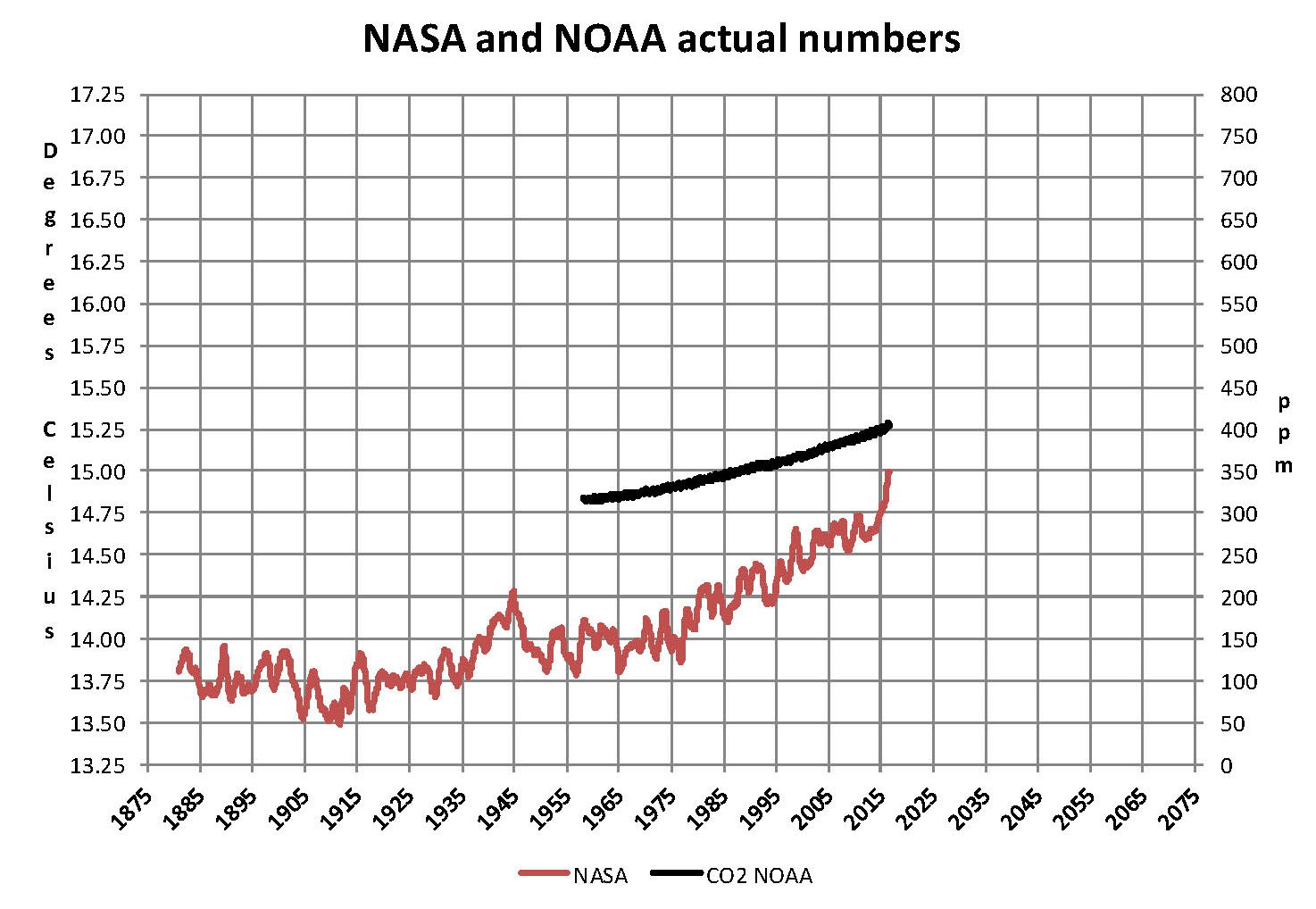
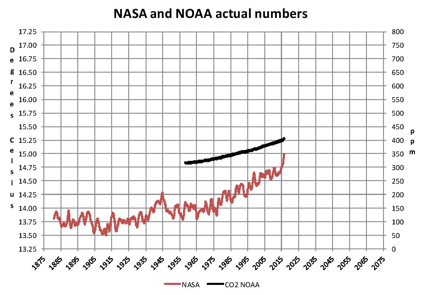
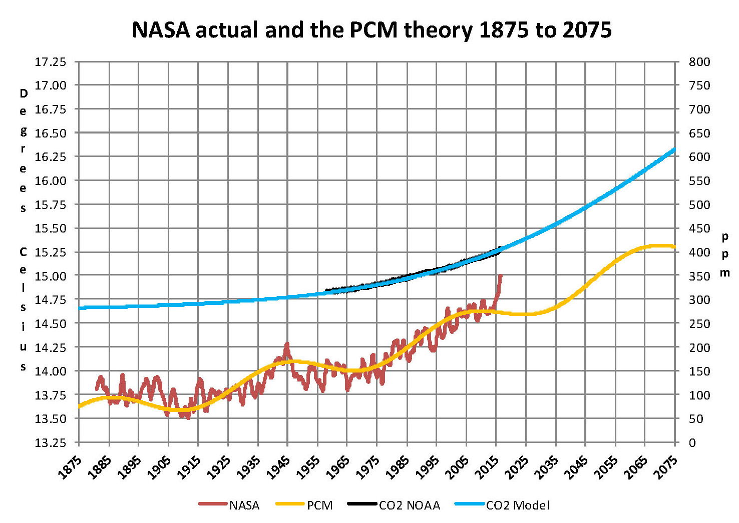
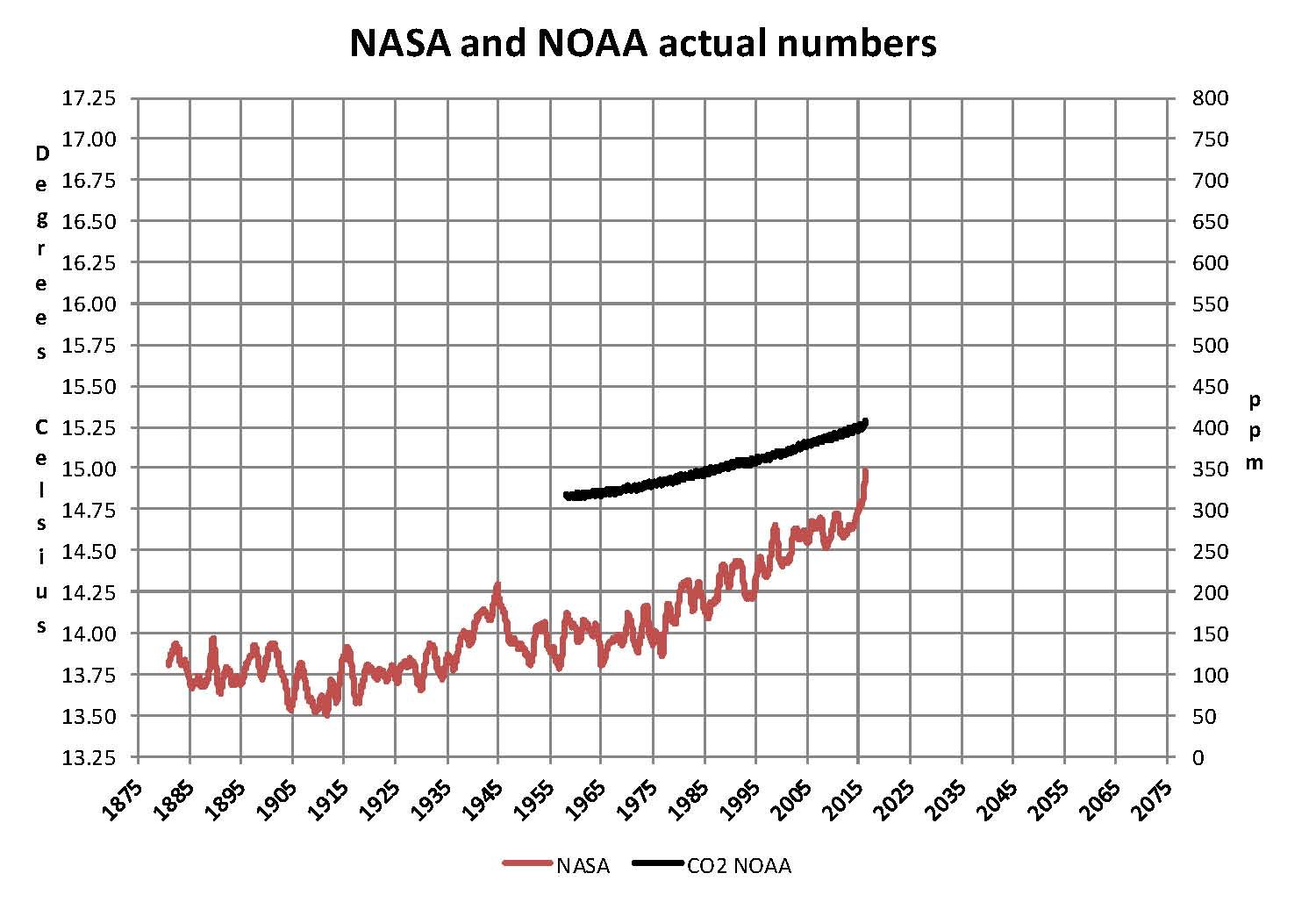
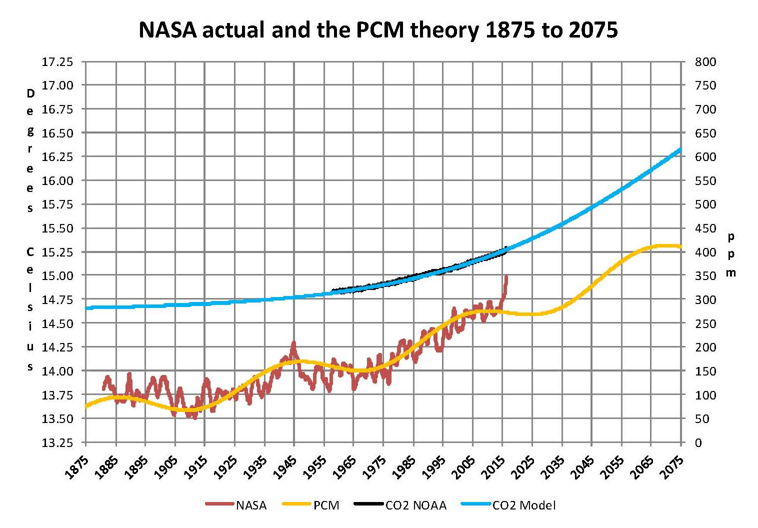
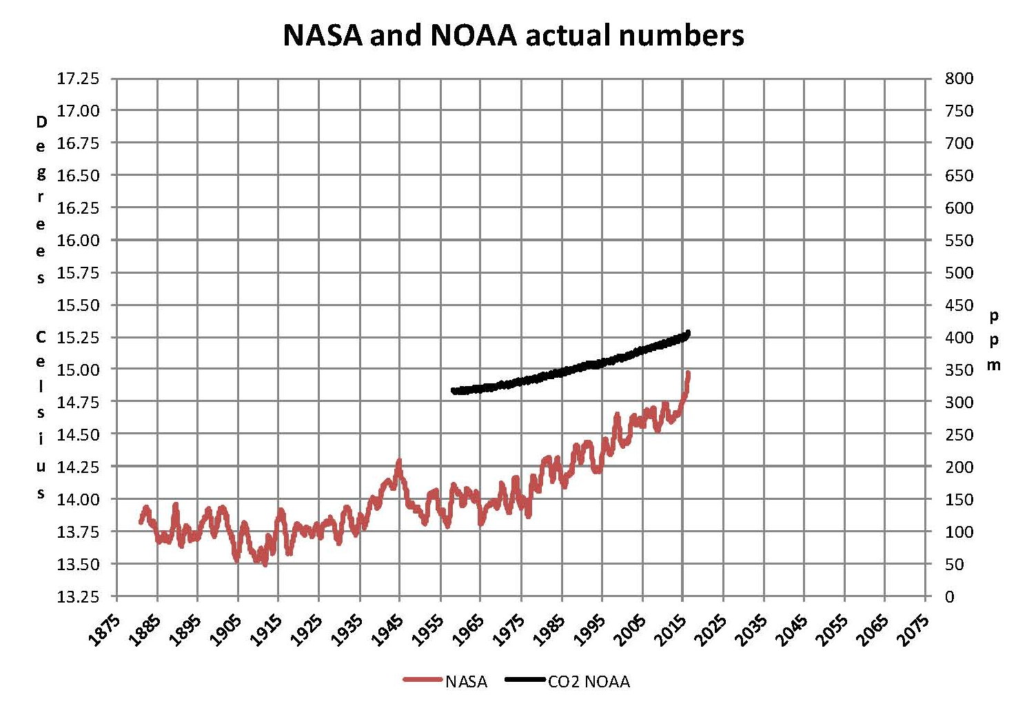
The analysis and plots shown here are based on the following two data series. First NASA-GISS estimates of a global temperature shown as an anomaly (converted to degrees Celsius) as shown in their table Land Ocean Temperature Index (LOTI) and shown in the following Chart as the red plot labeled NASA. This plot is shown as a twelve month moving average to minimize the large monthly swings and better show trends, the scale for the temperatures is on the left. Second NOAA-ESRL Carbon Dioxide (CO2) values in Parts Per Million (PPM) which are shown in the following Chart as a black plot labeled NOAA. This plot is shown exactly as the data from NOAA is presented and there is no need for a moving average the scale for CO2 is shown on the right.
NASA published data as stated in the first paragraph is shown as an anomaly, but what is a temperature anomaly? An anomaly is a deviation from some base value normally an average that is fixed. There were two problems with the system that NASA picked which were number one there is no “actual” global temperature and two since climate is a variable there cannot be a real base to measure from. NASA known for its science and engineering expertise back in the day thought it could get around these issues and created a system to do so. First they developed a computer model which took readings from all over the planet and made significant adjustments to them called homogenization and came up with the estimated global temperature. Second they picked the period 1950 to 1980 (30 years) and averaged the values and came up with 14.00 degrees Celsius and make that their base. Then they took the calculated temperature and subtracted the base from it which gave them the anomaly. The problem is that both the base and the anomaly are arbitrary.
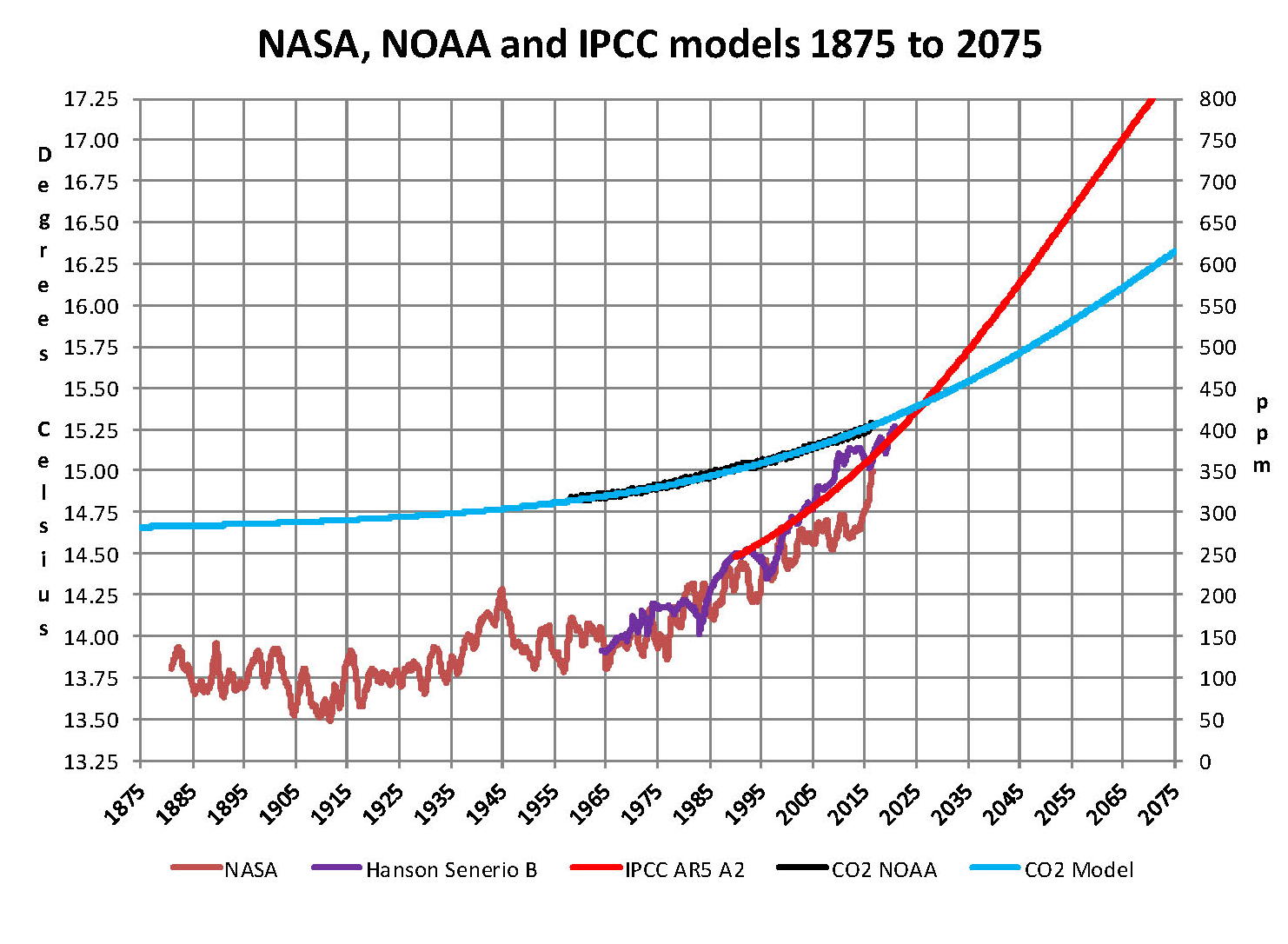
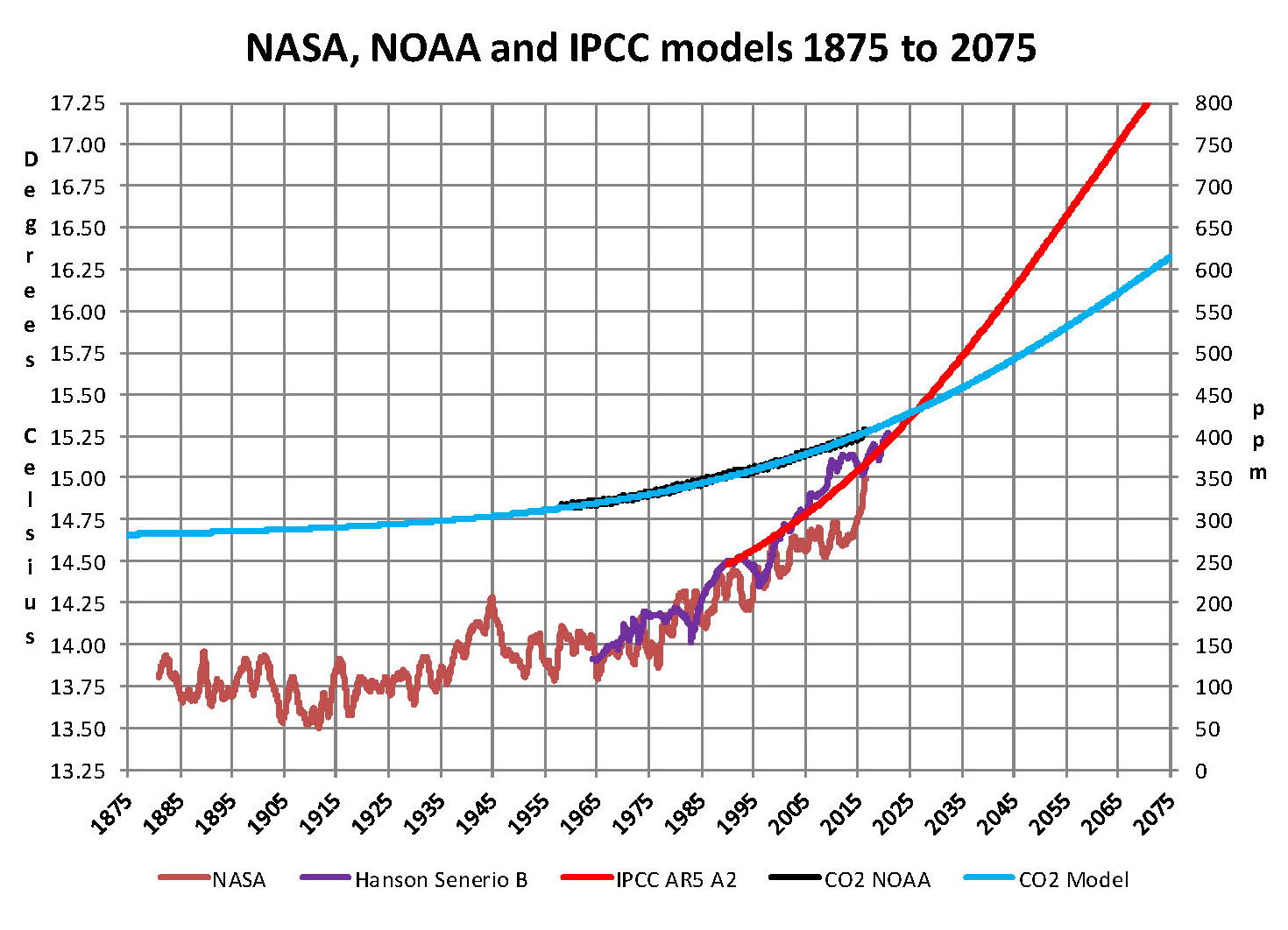
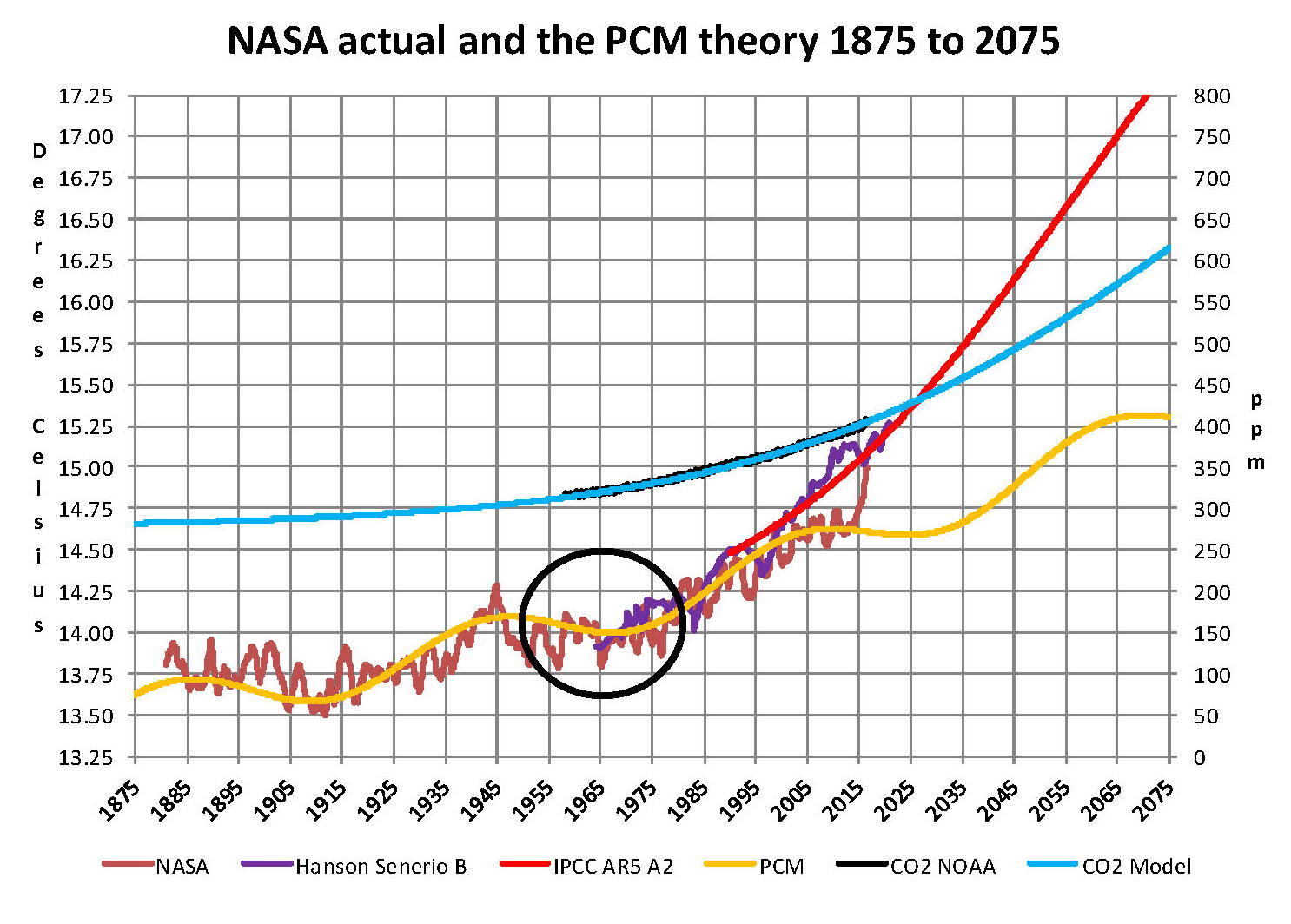
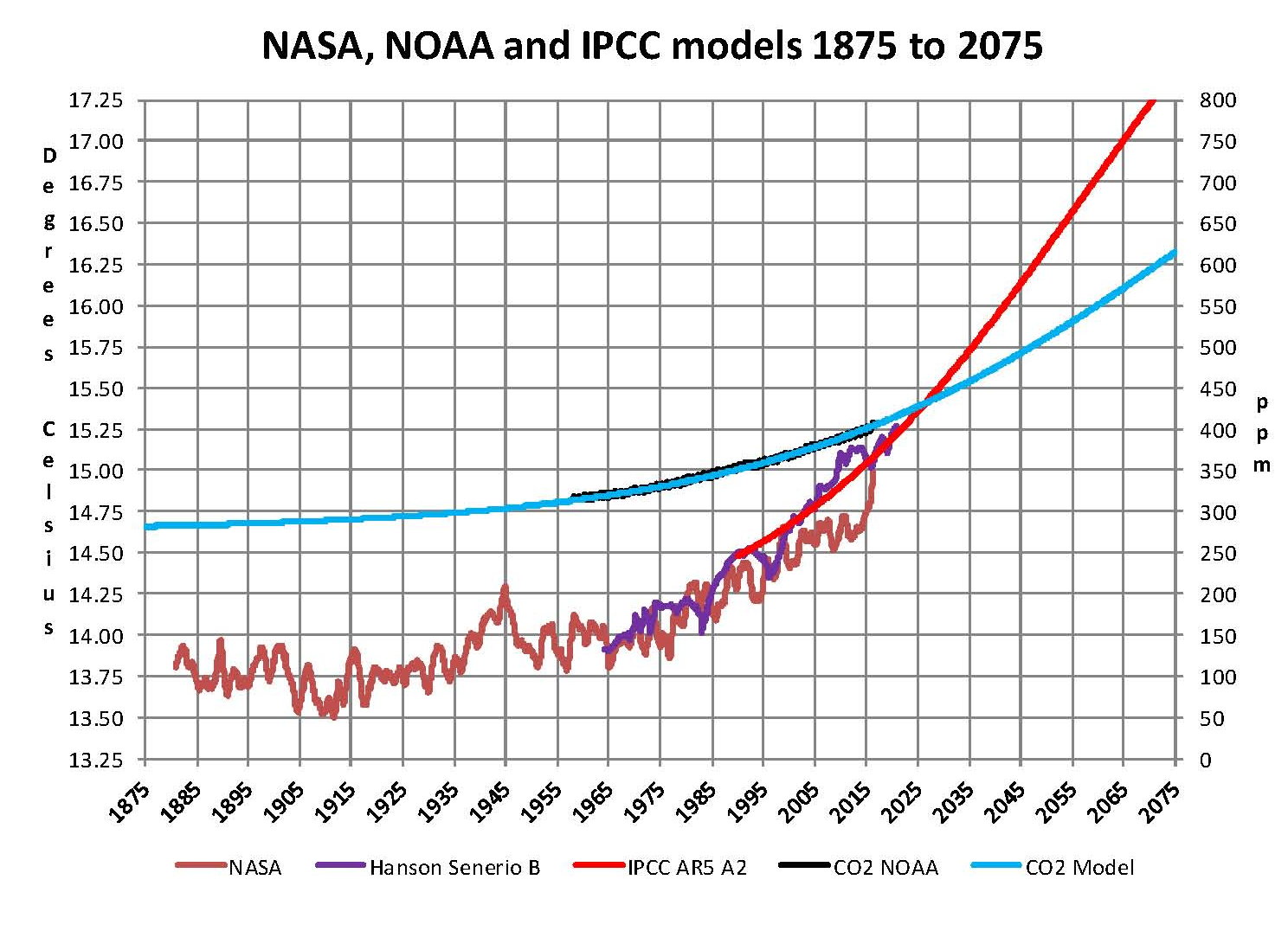
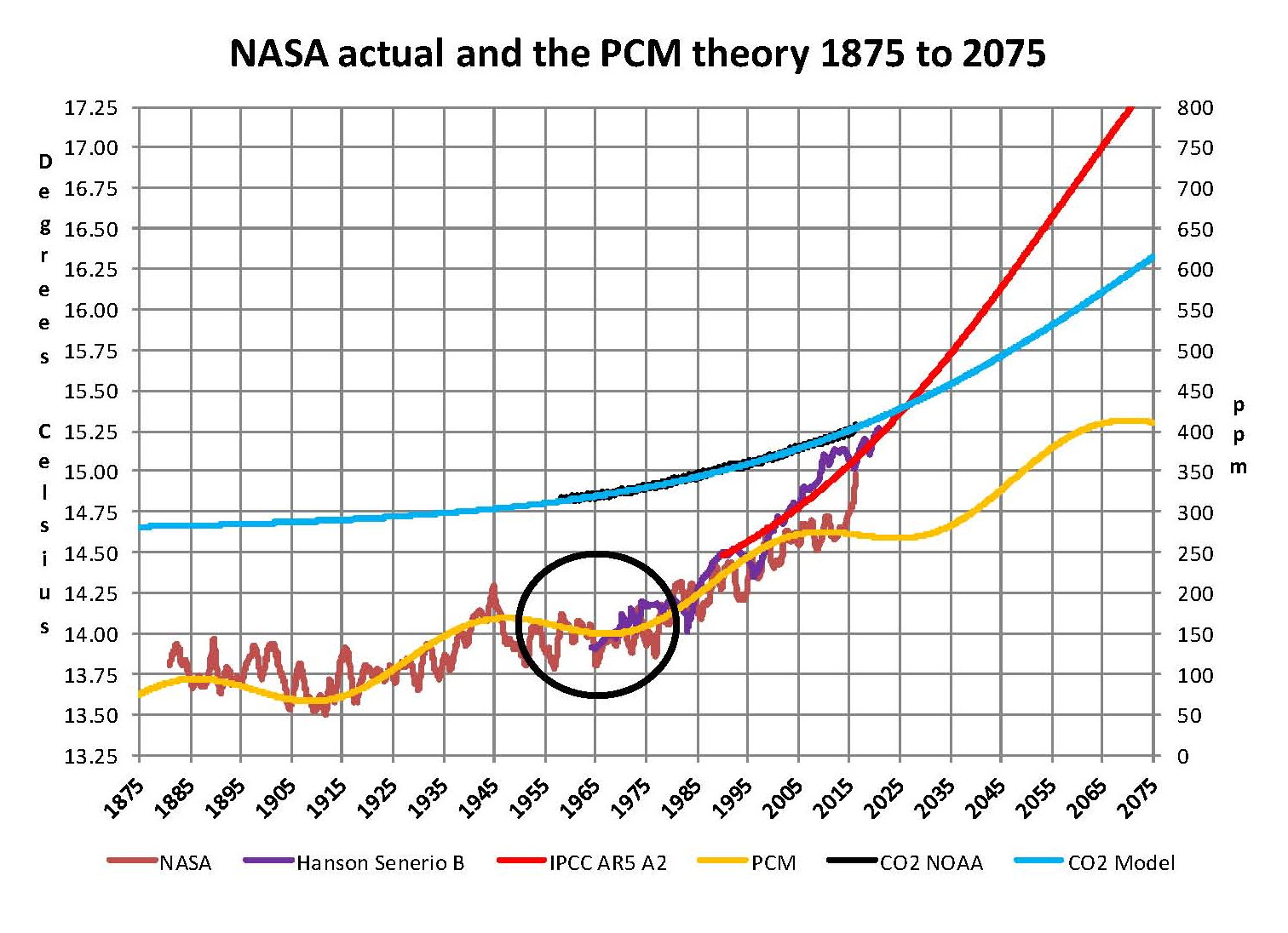
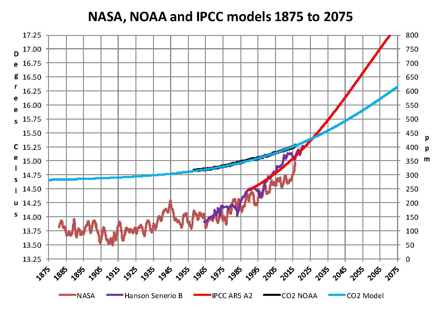
Now that we have a base to work with we are going to add to the previous Chart three things. The first is a trend line of the growth in CO2 since that is the entire basis for climate change according to the government through NASA and NOAA. That plot is superimposed over the black plot of the actual NOAA CO2 values as the cyan line labeled as the CO2 Model and one can see there is a very good fit to the actual NOAA values so there should be no dispute about its validity. This plot allows us to make projections as to future global temperatures according to the level of CO2. The second added item is James E. Hansen’s Scenario B data, which is the very core of the IPCC Global Climate models (GCM’s) and which was based on a CO2 sensitivity value of 3.0O Celsius per doubling of CO2. This plot is shown here in lavender and is part of a presentation that Hansen showed to congress in 1988 when the UN was about to set up the International Panel on Climate Change (IPCC) and this plot is labeled as Hansen Scenario B which Hansen stated was the most likely to happen based on his theories’. The third item is the current plot of the most likely temperature of the planet based on the growth of CO2 published by the IPCC. This plot is shown in Red and is labeled as IPCC AR5 A2 as that is the table where the data was found. This plot is a GCM computer projection of the planets temperature based to the complex relationships developed on the levels of CO2 by the IPCC through NASS and NOAA.
It can be seen in this Chart that the lavender plot and the Hansen plot are very close from 1965 to around 2000 after that, from 2000 to 2014, there is a very large and growing deviation reaching close to .5 degrees Celsius in 2014, which is not an insubstantial number. Also of note is that there doesn’t seem to be a good correlation between the growth in CO2 and the increase in the planets temperature. The CO2 is going up in a log function and the Temperature was going down in a log function until recently where it reversed and is now going up in a log function. That major change in direction that occurred between 2013 and 2014 is the subject of this paper.
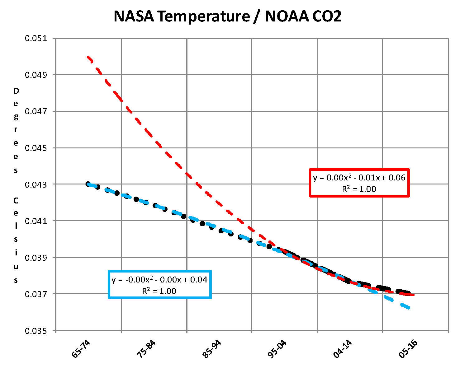
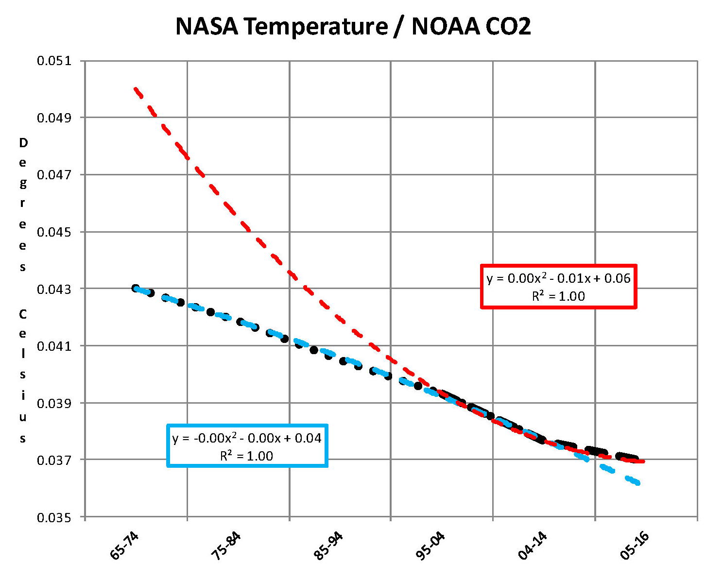
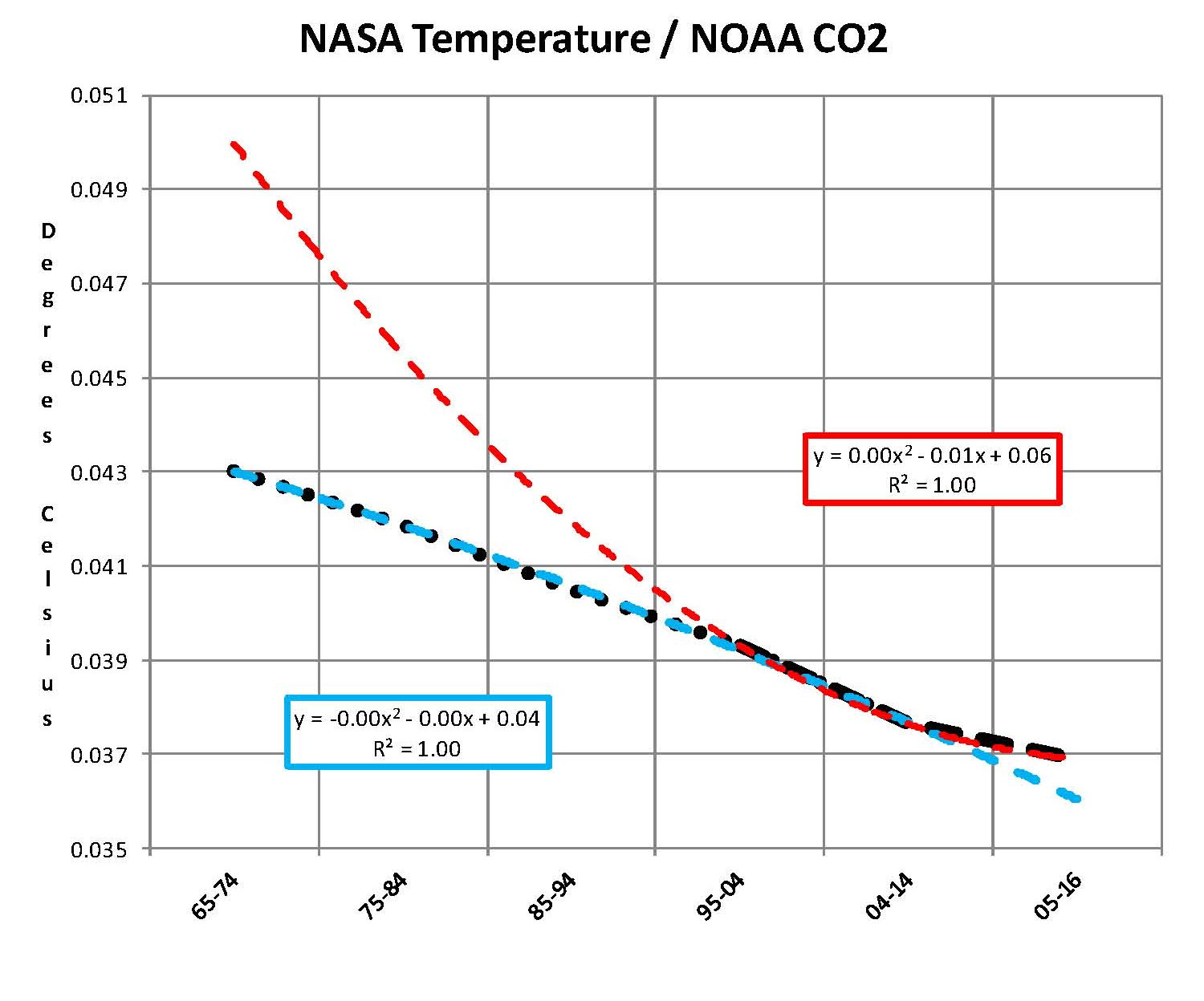
The next Chart is developed from the raw data from NASS and NOAA as shown in the first Chart. This plot was made first by adding ten years blocks of temperature and CO2 as indicated in the Chart and diving by 120 to give an average for each. Then the average Temperature was divided by the average CO2 to give degrees of temperature increase per PPM of CO2. After that was plotted it appeared that there were two different curves the first was from block 1965-1974 through block 2004-2014 shown as Black Dots and the second was from block 1995-2004 through block 2005-2016 shown as Black Dashes. When trend lines were added they were both almost perfect fits to the raw data and so you cannot see the data points very well on the Chart. These blocks were picked to represent the entire period of time where we had both NASA temperature data and NOAA Co2 levels.
On the following Chart are two sets of color coded information. The first is Cyan plot and the Cyan box with the equation in it along with the R2 value 0f 1.0 are for the first series from block 1965-1974 through block 2004-2014. The other is the Red plot and the Red box with the equation in it along with the R2 value of 1.0 which are for the first series from block 1965-1974 through block 2004-2016. We can speculate on how this change has happened but it cannot be said that the plot change is not real; however additions data over the next few years will be required to actually prove that something has changed.
In summary the Cyan data set indicates a diminishing effect of CO2 on global temperature for about 54 years and the Red data set represents an increasing effect of CO2 on global temperature for the past 2 years. Since both data sets have an R2 value of 1.00 the trend lines cannot be in question.
Before we get into a possible explanation to the drastic change from the Cyan data to the Red data that occurred in 20014 we need to consider other factors than CO2 on Climate change. The fault that occurred in the work that was done in the 1980’s was in assuming that there was an optimum or constant global temperature and therefore any change that was being observed was from the increasing amount of CO2 in the atmosphere. There may have been correlation but it was never proved that there was causation (high R2 value) between CO2 and global temperatures. With that assumption, which limited options, we moved from true science into the realm of political science. True science has an open mind and finds relationships that work in matching observations with predictions. Political science changes history and/or facts to match the desires of the politicians. Since the politicians control the money political science is what we get; which means that what we get may not be technically correct.
A decade ago when I started looking at “climate” change the first thing I did was look at geological temperature changes since it is well known that the climate is not a constant; I learned that 52 years ago in my undergrad geology and climatology courses in 1964. The next paragraph explains currently observed patterns in climate related to this subject.
Ignoring the last Ice Age which ended some 11,000 years ago when a good portion of the Northern hemisphere was under miles of ice the following observations give a starting point to any serious study on the subject. First, there is a clear up and down movement in global temperatures with a 1,000 some year cycle going back at least 3,000 to 4,000 years; probably because of the apsidal precession of the earth’s orbit of about 20,000 years for a complete cycle. However about every 10,000 years the seasons are reversed making the winter colder and the summer warmer in the northern hemisphere. 10,000 years from now the seasons will be reversed. Secondly, there are also 60 to 70 year cycles in the Pacific and the Atlantic oceans that are well documented. These are known as the Atlantic MultiDecadal Oscillations (AMO) in the Atlantic and as La Nina and El Nino in the Pacific. Thirdly, we also know that there are greenhouse gases such as carbon dioxide that can affect global temperatures. Lastly the National Academy of Sciences (NAS) estimated that carbon dioxide had a doubling rate of 3.0O Celsius plus or minus 1.5O Celsius in 1979 when there were only two studies available and one for sure and maybe both were not per reviewed.
The result of looking objectively at the three possible sources of global temperature changes was a series of equations based on these observations that when added together produced a sinusoidal curve that seemed to follow NASA published temperatures very closely. Since this curve was based on observed temperature patterns it was called a Pattern Climate Model (PCM) which has been described in previous papers and posts on my blog and since it is generated by “equations” many assume it is some form of least squares curve fitting, which it is not. It does seem to be related to ocean currents.
As can be seen in the following Chart the PCM there is a 69.1 year cycle that moves the trend line up and then down a total of 0.29O Celsius and we are now in the downward portion of that trend (-.01491O C per year) which will continue until around ~2035. This short cycle is clearly observed in the raw NASA data in the LOTI table going back to 1880. Then there is a long trend, 1036.7 years with an up and down of 1.65O Celsius (.00396O C per year) also observed in the NASA data. Lastly, there is CO2 adding about .0079O Celsius per year so currently they all basically wash out at -.0039O C per year, which matches the current holding pattern we are experiencing. After about 2035 the short cycle will have bottomed and turn up and all three will be on the upswing again. Note: the values shown here are only representative as the actual model uses many more places than what are shown here.
When using the 12 month running average for global temperatures up until 2014 the PCM model was within +/- .01 degrees of what NASA was publishing in their LOTI table since the early 1960’s as shown in the next Chart. Further the back projection of the PCM plot matched historical records and global temperatures going back past the time of Christ. It should also be consider that geologically CO2 levels have reached levels many times that of the current 400 ppm without destroying the planet so the current hysteria over the current small numbers can only be explained by political science not real science.

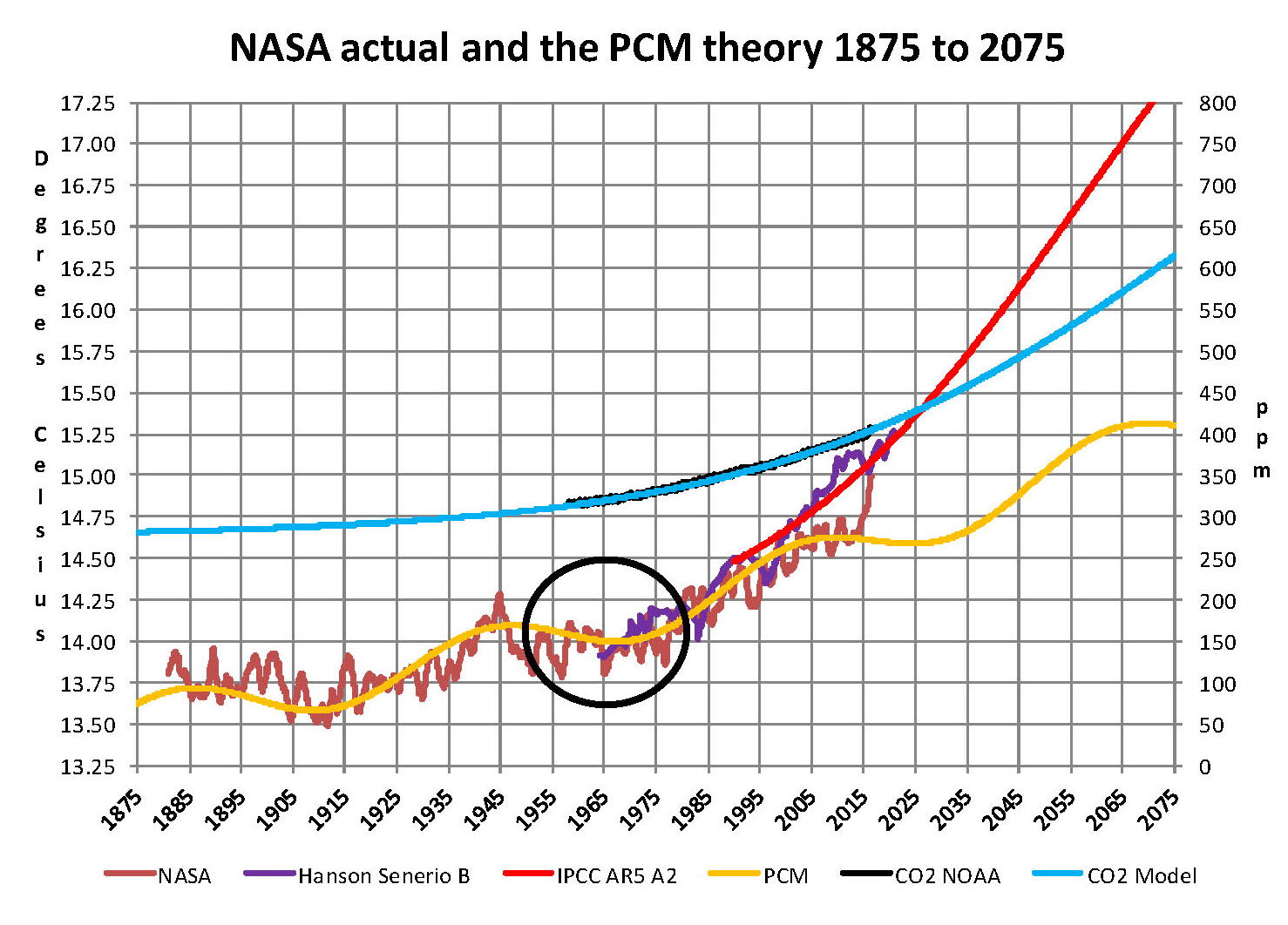
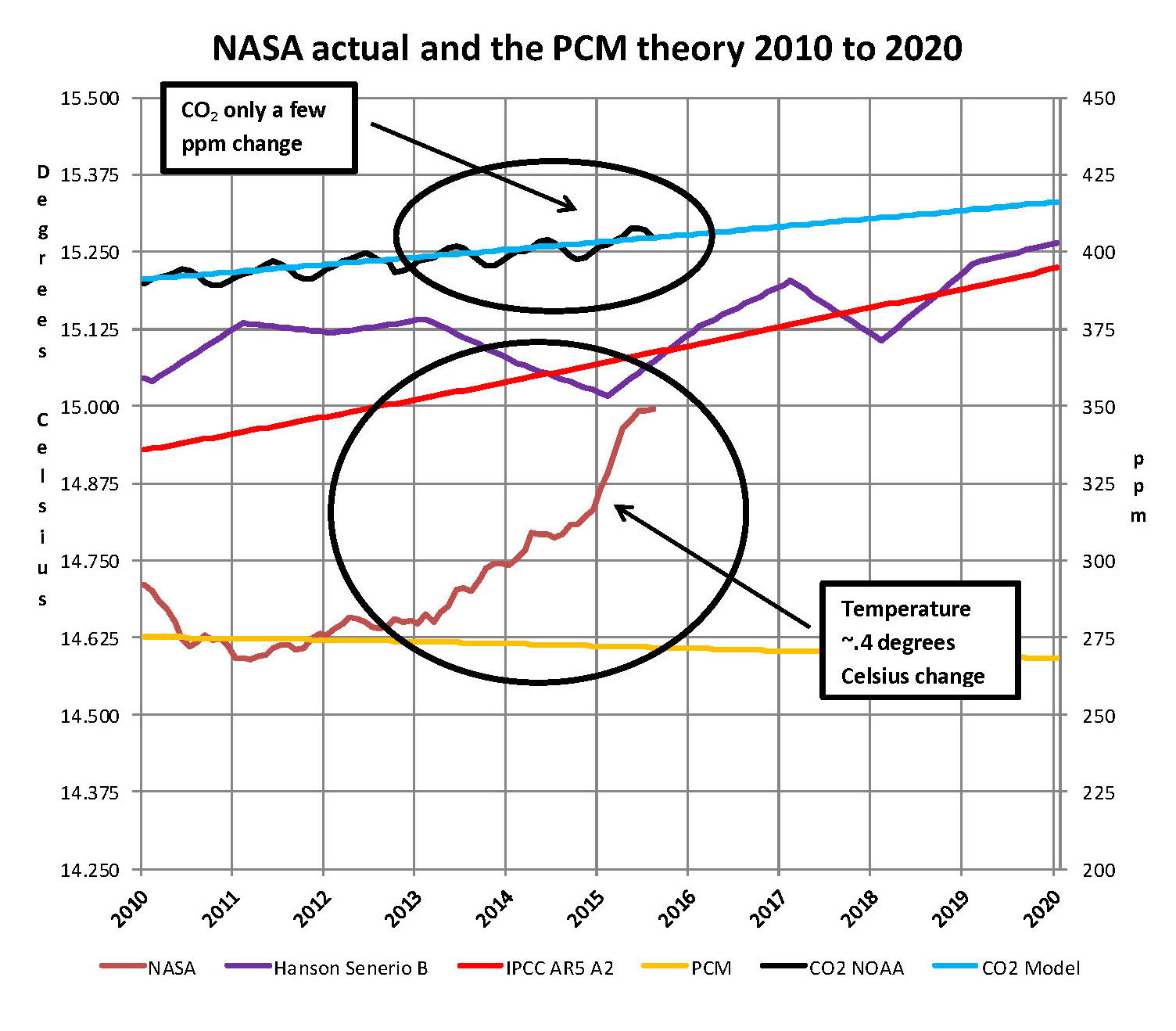
The nest step in this analysis is to put all of the known data and projections into one Chart which will contain: NASA’s table LOTI global temperature estimates, NOAA’s actual CO2 values, the CO2 model projections, the PCM model global temperature plot, Hansen’s Scenario B 1988 global temperature plot, and lastly the IPCC AR5 A2 global temperature plot. With that done we can look at the results and try to make some sense of what is going on with the various arms of the federal government that are promoting that carbon based fuels be eliminated since they are responsible for the global temperature level going up. As previously started when the government pours money into the sciences the sciences respond with technical papers the support the governments views, this is what I call political science verses real science as was done prior to the 1980’s; money talks and BS walks as everyone on the street knows. This Chart views a good overview of the current situation showing all the facts and all the projections.
This Chart contains no manipulation of the data and the only change that was made was to convert the NASA anomalies back to degrees Celsius to make it more readable to lay people. This is only a change in units and has no bearing on the look. A subject not broached here is that of the NASA homogenization process itself and the base period from 1950 to 1980. The portion in the black circle contains the NASA base period of 14.00 degrees Celsius and the reason it’s brought up here is that the Homogenization process causes the global temperatures to move around since the entire data base all the way back to 1880 is recalculated each month. But since the base has to stay at 14.00 degrees Celsius the program must be set to not allow changes in that period of time. I’m sure the programmers have fun with that. Prior work here has shown how this creates a teeter totter effect with the data plots, some of which have recently been significant.
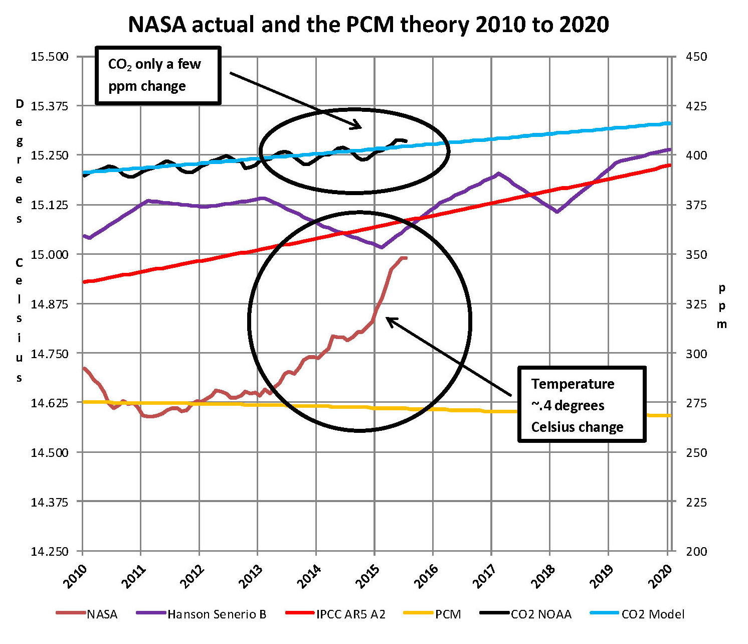
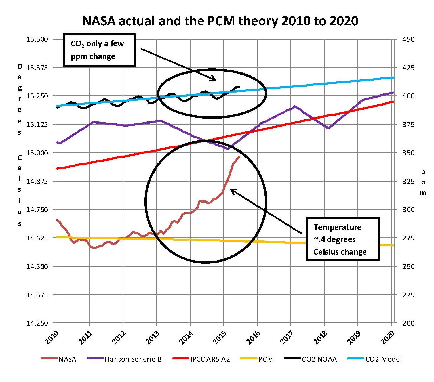
The next Chart will be a look at the period from 2010 to 2020 so we can see the detail of the past few years where a change in CO2 of only a few ppm has caused a major change in the global temperature way beyond anything previously shown in any published NASA data. There are two black ovals on the Chart one at the top of the Chart which is a black oval around the CO2 levels for 2013, 2014, 2015 and part of 2016 and it’s very obvious that there has been very little change, maybe 4 ppm or about 1%. Then at the bottom of the Chart is another black oval around the NASA global temperature levels for 2013, 2014, 2015 and part of 2016 and its very obvious that there has been a very large change, almost .40 degrees Celsius or about 2.7%. There has never been such a large increase in temperature from such a small increase in CO2.
By contrast the previous comparable period of the last part of 2010 through 2013 shows about the same increase for CO2 at 1.1% but no increase for global temperature but actually small decrease. Worse it appears that this current strange upward trend will continue as the values shown here are based on a 12 month moving average and the current values being published by NASA have been very high for the past 7 months and therefore I would expect the NASA plot to be well over 15.00 Celsius within a few months and certainly before the end of 2016. Also in looking at the raw data for September 2015 and October 2015 there was a jump of almost .300 Celsius that is a very large number for a couple of months and as we have shown here in previous charts not reasonable at all and therefore a perfect example of political science.
In summary, the IPCC models were designed before a true picture of the world’s climate was understood. During the 1980’s and 1990’s CO2 levels were going up and the world temperature was also going up so there appeared to be correlation and causation. The mistake that was made was looking at only a ~20 year period when the real variations in climate all move in much longer cycles of decades and centuries. Those other cycles can be observed in the NASA data but they were ignored for some reason. By ignoring those trends and focusing only on CO2 the models will be unable to correctly plot global temperatures until they are fixed.
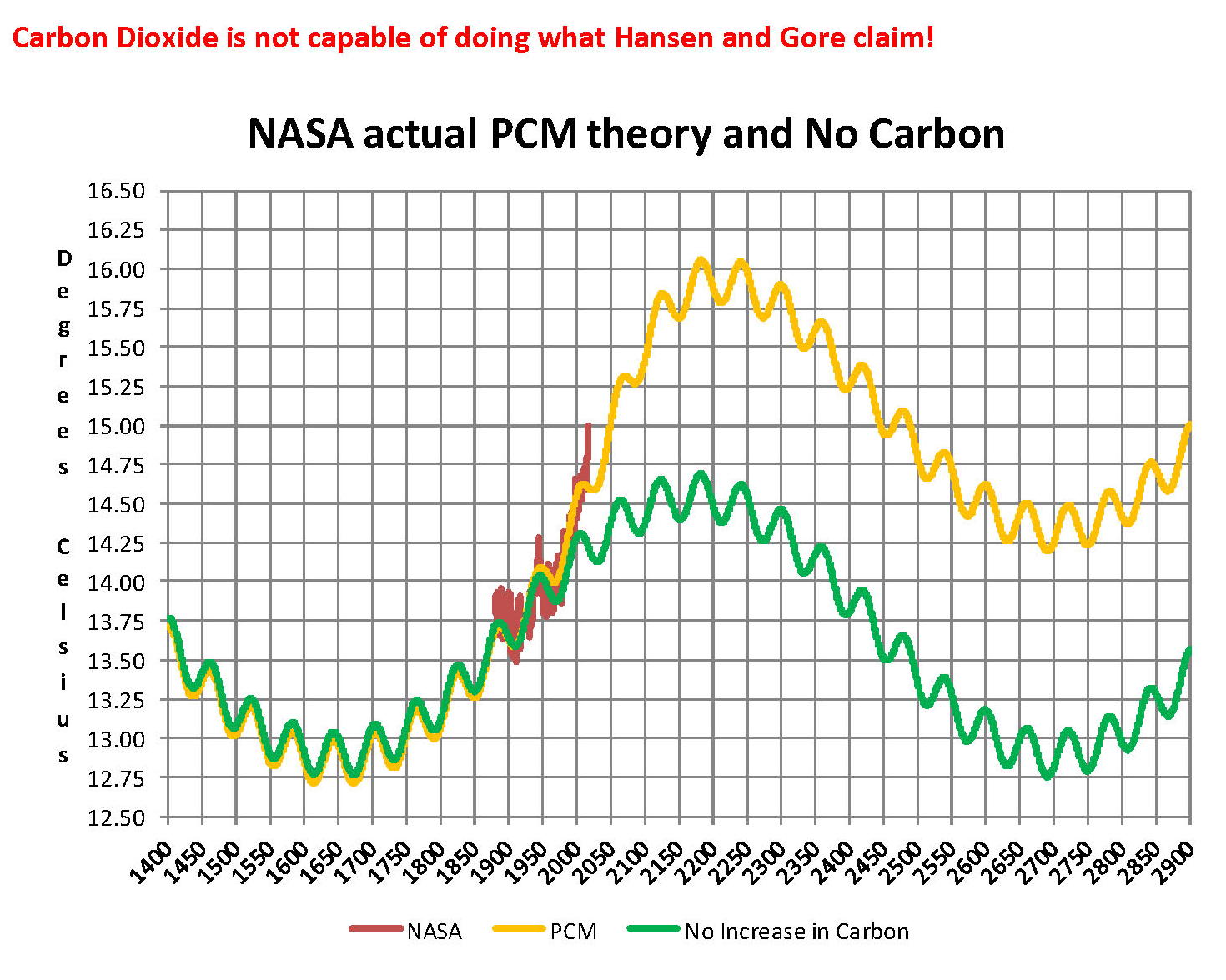
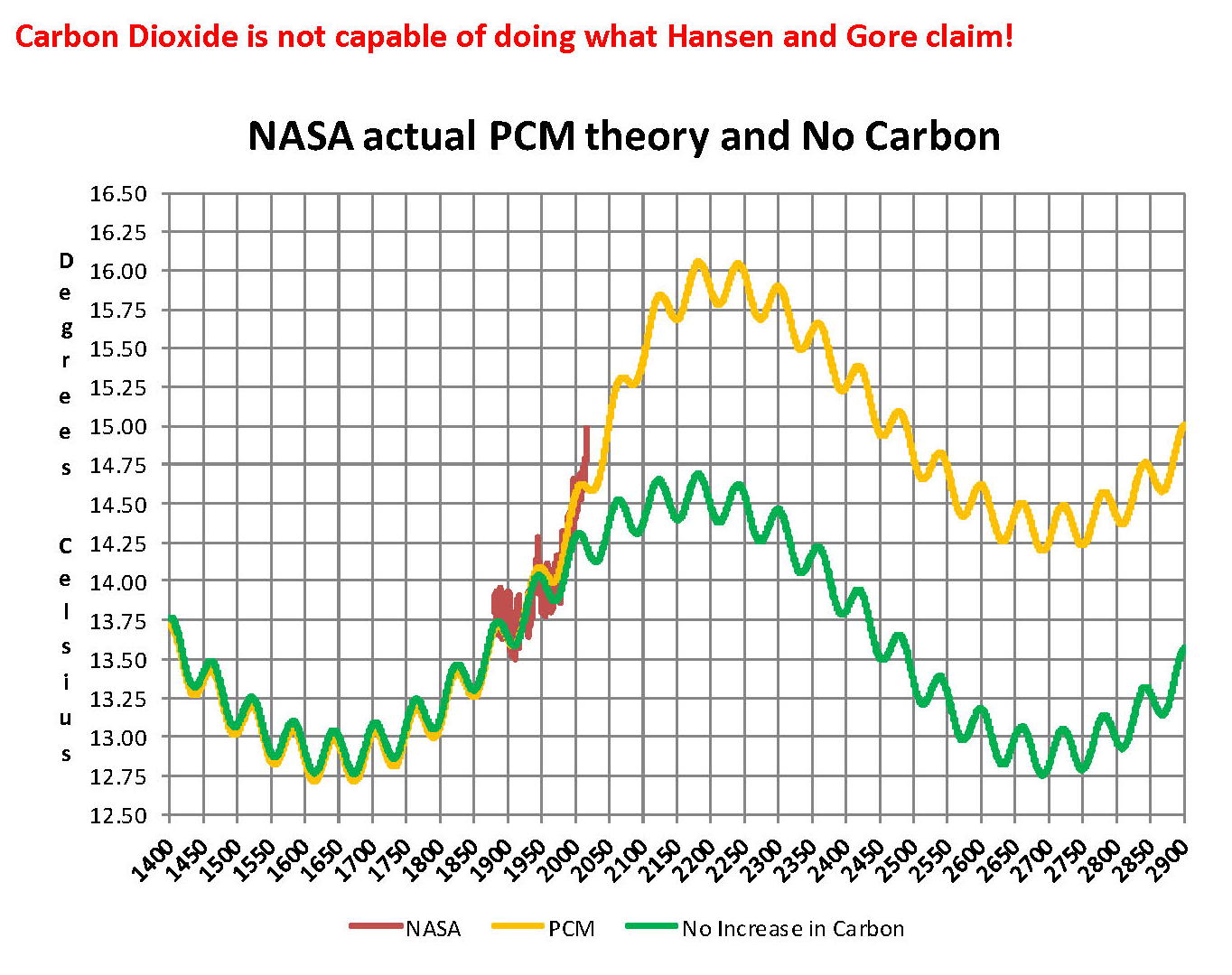
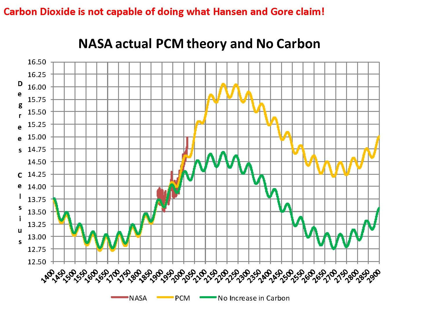
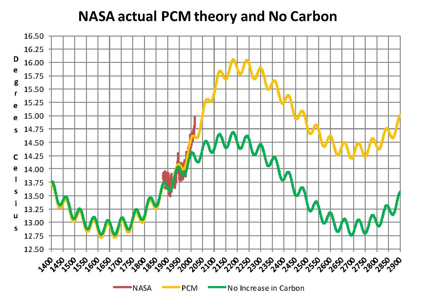
Lastly, the next chart shows what a plot of the PCM model, in yellow, would look like from the year 1400 to the year 2900. This plot matches reasonably well with recorded history and fits the current NASA-GISS table LOTI data, in red, very closely, despite homogenization. I understand that this model is not based on physics but it is also not true curve fitting. It’s based on observed reoccurring patterns in the climate. These patterns can be modeled and when they are, you get a plot that works better than any of the IPCC’s GCM’s. If the conditions that create these patterns do not change and CO2 continues to increase to 800 ppm or even 1000 ppm than this model will work well into the foreseeable future. 150 years from now global temperatures will peak at around 15.750 to 16.000 C and then will be on the downside of the long cycle for the next ~500 years.
The overall effect of CO2 reaching levels of 1000 ppm or even higher will be about 1.50 C which is about the same as that of the long cycle. The Green plot on the Chart shows the observed pattern with no change in CO2 from the pre-industrial era of ~280 ppm. CO2 cannot affect global temperatures more than 1.500 C +/- no matter what the ppm level of CO2is. The reason being that the CO2 sensitivity value is not 3.00 per doubling of CO2 but under 1.00 C per doubling of CO2 as shown in morecurrent scientific work.
The purpose of this post is to make people aware of the errors inherent in the IPCC models so that they can be corrected.
The Obama administration’s “need” for a binding UN climate treaty with mandated CO2 reductions in Europe and America was achieved as predicted at the COP12 conference in Paris in December 2015. To support this endeavor NASA was forced to show ever increasing global temperatures that will make less and less sense based on observations and satellite data which will all be dismissed or ignored. Within a few years the manipulation will be obvious even to those without knowledge in the subject, but by then it will be to late the damage to the reputation of science will have been done.
Sir Karl Raimund Popper (28 July 1902 – 17 September 1994) was an Austrian and British philosopher and a professor at the London School of Economics. He is considered one of the most influential philosophers for science of the 20th century, and he also wrote extensively on social and political philosophy. The following quotes of his apply to this subject.
If we are uncritical we shall always find what we want: we shall look for, and find, confirmations, and we shall look away from, and not see, whatever might be dangerous to our pet theories.
Whenever a theory appears to you as the only possible one, take this as a sign that you have neither understood the theory nor the problem which it was intended to solve.
… (S)cience is one of the very few human activities — perhaps the only one — in which errors are systematically criticized and fairly often, in time, corrected.
The analysis and plots shown here are based on the following two data series. First NASA-GISS estimates of a global temperature shown as an anomaly (converted to degrees Celsius) as shown in their table Land Ocean Temperature Index (LOTI) and shown in the following Chart as the red plot labeled NASA. This plot is shown as a twelve month moving average to minimize the large monthly swings and better show trends the scale for the temperatures is on the left. Second NOAA-ESRL Carbon Dioxide (CO2) values in Parts Per Million (PPM) which are shown in the following Chart as a black plot labeled NOAA. This plot is shown exactly as the data from NOAA is presented and there is no need for a moving average the scale for CO2 is shown on the right.
NASA published data as stated in the first paragraph is shown as an anomaly, but what is a temperature anomaly? An anomaly is a deviation from some base value normally an average that is fixed. There were two problems with the system that NASA picked which were number one there is no “actual” global temperature and two since climate is a variable there cannot be a real base to measure from. NASA known for its expertise back in the day thought it could get around these issues and created a system to do so. First they developed a computer model which took readings from all over the planet and made adjustments to them called homogenization and came up with the estimated global temperature. Second they picked the period 1950 to 1980 (30 years) and averaged the values and came up with 14.00 degrees Celsius and make that their base. Then they took that temperature and subtracted the base from it which gave them the anomaly. The problem is that both the base and the anomaly are arbitrary.
Now that we have a base to work with we are going to add to the previous Chart three things. The first is a trend line of the growth in CO2 since that is the entire basis for climate change according to the government through NASA and NOAA. That plot is superimposed over the black plot of the actual NOAA CO2 values as the cyan line labeled as the CO2 Model and one can see there is a very good fit to the actual NOAA values so there should be no dispute about its validity. This plot allows us to make projections as to future global temperatures according to the science. The second added item is James E. Hansen’s Scenario B data, which is the very core of the IPCC Global Climate models (GCM’s) and which was based on a CO2 sensitivity value of 3.0O Celsius per doubling of CO2. This plot is shown here in lavender and is part of a presentation that Hansen showed to congress in 1988 when the UN was about to set up the International Panel on Climate Change (IPCC) and this plot is labeled as Hansen Scenario B which Hansen stated was the most likely to happen based on his theories’. The third item is the current plot of the most likely temperature of the planet based on the growth of CO2 published by the IPCC. This plot is shown in Red and is labeled as IPCC AR5 A2 as that is the table where the data was found. This plot is a GCM computer projection of the planets temperature based to the complex relationships developed on the levels of CO2 by the IPCC through NASS and NOAA.
It can be seen in this Chart that the lavender plot and the Hansen plot are very close from 1965 to around 2000 after that, from 2000 to 2014, there is a very large and growing deviation reaching close to .5 degrees Celsius in 2014, which is not an insubstantial number. Also of note is that there doesn’t seem to be a good correlation between the growth in CO2 and the increase in the planets temperature. The CO2 is going up in a log function and the Temperature was going down in a log function until recently where it reversed and is now going up in a log function. That major change in direction that occurred in 20014 is the subject of this paper.
The next Chart is developed from the raw data from NASS and NOAA as shown in the first Chart. This plot was made first by adding ten years blocks of temperature and CO2 as indicated in the Chart and diving by 120 to give an average for each. Then the average Temperature was divided by the average CO2 to give degrees of temperature increase per PPM of CO2. After that was plotted it appeared that there were two different curves the first was from block 1965-1974 through block 2004-2014 shown as Black Dots and the second was from block 1995-2004 through block 2005-2016 shown as Black Dashes. When trend lines were added they were both almost perfect fits to the raw data and so you cannot see the data points very well on the Chart. These blocks were picked to represent the entire period of time where we had both NASA temperature data and NOAA Co2 levels.
On the following Chart are two sets of color coded information. The first is Cyan plot and the Cyan box with the equation in it along with the R2 value 0f 1.0 are for the first series from block 1965-1974 through block 2004-2014. The other is the Red plot and the Red box with the equation in it along with the R2 value of 1.0 which are for the first series from block 1965-1974 through block 2004-2016. We can speculate on how this change has happened but it cannot be said that the plot change is not real; however additions data over the next few years will be required to actually prove that something has changed.
In summary the Cyan data set indicates a diminishing effect of CO2 on global temperature for about 54 years and the Red data set represents an increasing effect of CO2 on global temperature for the past 2 years. Since both data sets have an R2 value of 1.00 the trend lines cannot be in question.
Before we get into a possible explanation to the drastic change from the Cyan data to the Red data that occurred in 20014 we need to consider other factors than CO2 on Climate change. The fault that occurred in the work that was done in the 1980’s was in assuming that there was an optimum or constant global temperature and therefore any change that was being observed was from the increasing amount of CO2 in the atmosphere. There may have been correlation but it was never proved that there was causation (high R2 value) between CO2 and global temperatures. With that assumption which limited options we moved from true science into the realm of political science. True science has an open mind and finds relationships that work in matching observations with predictions. Political science changes history and/or facts to match the desires of the politicians. Since the politicians control the money political science is what we get; which means that what we get may not be technically correct.
A decade ago when I started looking at “climate” change the first thing I did was look at geological temperature changes since it is well known that the climate is not a constant; I learned that 52 years ago in my undergrad geology and climatology courses in 1964. The next paragraph explains currently observed patterns in climate related to this subject.
Ignoring the last Ice Age which ended some 11,000 years ago when a good portion of the Northern hemisphere was under miles of ice the following observations give a starting point to any serious study on the subject. First, there is a clear up and down movement in global temperatures with a 1,000 some year cycle going back at least 3,000 to 4,000 years; probably because of the apsidal precession of the earth’s orbit of about 20,000 years for a complete cycle. However about every 10,000 years the seasons are reversed making the winter colder and the summer warmer in the northern hemisphere. 10,000 years from now the seasons will be reversed. Secondly, there are also 60 to 70 year cycles in the Pacific and the Atlantic oceans that are well documented. These are known as the Atlantic MultiDecadal Oscillations (AMO) in the Atlantic and as La Nina and El Nino in the Pacific. Thirdly, we also know that there are greenhouse gases such as carbon dioxide that can affect global temperatures. Lastly the National Academy of Sciences (NAS) estimated that carbon dioxide had a doubling rate of 3.0O Celsius plus or minus 1.5O Celsius in 1979 when there were only two studies available and one for sure and maybe both were not per reviewed.
The result of looking objectively at the three possible sources of global temperature changes was a series of equations based on these observations that when added together produced a sinusoidal curve that seemed to follow NASA published temperatures very closely. Since this curve was based on observed temperature patterns it was called a Pattern Climate Model (PCM) which has been described in previous papers and posts on my blog and since it is generated by “equations” many assume it is some form of least squares curve fitting, which it is not. It does seem to be related to ocean currents.
As can be seen in the following Chart the PCM there is a 69.1 year cycle that moves the trend line up and then down a total of 0.29O Celsius and we are now in the downward portion of that trend (-.01491O C per year) which will continue until around ~2035. This short cycle is clearly observed in the raw NASA data in the LOTI table going back to 1880. Then there is a long trend, 1036.7 years with an up and down of 1.65O Celsius (.00396O C per year) also observed in the NASA data. Lastly, there is CO2 adding about .0079 degrees Celsius per year so they all basically wash out at -.0039 O C per year, which matches the current holding pattern we are experiencing. After about 2035 the short cycle will have bottomed and turn up and all three will be on the upswing again. Note: the values shown here are only representative as the actual model uses many more places than what are shown here.
When using the 12 month running average for global temperatures up until 2014 the PCM model was within +/- .01 degrees of what NASA was publishing in their LOTI table since the early 1960’s as shown in the next Chart. Further the back projection of the PCM plot matched historical records and global temperatures going back past the time of Christ. It should also be consider that geologically CO2 levels have reached levels many times that of the current 400 ppm without destroying the planet so the current hysteria over the current small numbers can only be explained by political science not real science.
The nest step in this analysis is to put all of the known data and projections into one Chart which will contain: NASA’s table LOTI global temperature estimates, NOAA’s actual CO2 values, the CO2 model projections, the PCM model global temperature plot, Hansen’s Scenario B 1988 global temperature plot, and lastly the IPCC AR5 A2 global temperature plot. With that done we can look at the results and try to make some sense of what is going on with the various arms of the federal government that are promoting that carbon based fuels be eliminated since they are responsible for the global temperature level going up. As previously started when the government pours money into the sciences the sciences respond with technical papers the support the governments views, this is what is call political science verses real science as was done prior to the 1980’s; money talks and BS walks as everyone on the street knows. This Chart views a good overview of the current situation showing all the facts and all the projections.
This Chart contains no manipulation of the data and the only change that was made was to convert the NASA anomalies back to degrees Celsius to make it more readable to lay people. This is only a change in units and has no bearing on the look. A subject not broached here is that of the NASA homogenization process itself and the base period from 1950 to 1980. The portion in the black circle contains the NASA base period of 14.00 degrees Celsius and the reason it’s brought up here is that the Homogenization process causes the global temperatures to move around since the entire data base all the way back to 1880 is recalculated. But since the base has to stay at 14.00 degrees Celsius the program must be set to not allow changes in that period of time. I’m sure the programmers have fun with that. Prior work here has shown how this creates a teeter totter effect with the data plots, some of which have recently been significant.
The next Chart will be a look at the period from 2010 to 2020 so we can see the detail of the past few years where a change in CO2 of only a few ppm has caused a major change in the global temperature way beyond anything previously shown in any published NASA data. There are two black ovals on the Chart one at the top of the Chart which is a black oval around the CO2 levels for 2014, 2015 and part of 2016 and it’s very obvious that there has been very little change, maybe 4 ppm or about 1%. Then at the bottom of the Chart is another black oval around the NASA global temperature levels for 2014, 2015 and part of 2016 and its very obvious that there has been a very large change, maybe .33 degrees Celsius or about 2.2%. There has never been such a large increase in temperature from such a small increase in CO2.
By contrast the previous comparable period of the last part of 2010 through 2013 shows about the same for CO2 at 1.1% but only a .2% increase for global temperature, basically flat. Worse it appears that this upward trend will continue as these values are based on a 12 month moving average and the current values being published by NASA have been very high for the past 6 months and so I would expect the NASA plot to be well over 15.00 degrees Celsius within a few months. In looking at the raw data for September 2015 and October 2015 there is a jump of about .25 degrees Celsius that is a very large number for one month and as we have shown here in a previous chart not reasonable at all and a perfect example of political science.
In summary, the IPCC models were designed before a true picture of the world’s climate was understood. During the 1980’s and 1990’s CO2 levels were going up and the world temperature was also going up so there appeared to be correlation and causation. The mistake that was made was looking at only a ~20 year period when the real variations in climate all move in much longer cycles. Those other cycles can be observed in the NASA data but they were ignored for some reason. By ignoring those trends and focusing only on CO2 the models will be unable to correctly plot global temperatures until they are fixed.
Lastly, the next chart shows what a plot of the PCM model, in yellow, would look like from the year 1400 to the year 2900. The plot matches reasonably well with history and fits the current NASA-GISS table LOTI data, in red, very closely, despite homogenization. I understand that this model is not based on physics but it is also not curve fitting. It’s based on observed reoccurring patterns in the climate. These patterns can be modeled and when they are, you get a plot that works better than any of the IPCC’s GCM’s. If the conditions that create these patterns do not change and CO2 continues to increase to 800 ppm or even 1000 ppm than this model will work into the foreseeable future. 150 years from now global temperatures will peak at around 15.75 to 16.00 degrees C and then will be on the downside of the long cycle for the next 500 years. The overall effect of CO2 reaching levels of 1000 ppm or even higher will be about 1.5 degrees C which is about the same as that of the long cycle. The Green plot on the Chart shows the observed pattern with no change in CO2 from the pre-industrial era of ~280 ppm.
The purpose of this post is to make people aware of the errors inherent in the IPCC models so that they can be corrected.
The Obama administration’s “need” for a binding UN climate treaty with mandated CO2 reductions in Europe and America was achieved as predicted at the COP12 conference in Paris in December 2015. To support this endeavor NASA was forced to show ever increasing global temperatures that will make less and less sense based on observations and satellite data which will all be dismissed or ignored. Within a few years the manipulation will be obvious even to those without knowledge in the subject, but by then it will be to late the damage to the reputation of science will have been done.
Sir Karl Raimund Popper (28 July 1902 – 17 September 1994) was an Austrian and British philosopher and a professor at the London School of Economics. He is considered one of the most influential philosophers for science of the 20th century, and he also wrote extensively on social and political philosophy. The following quotes of his apply to this subject.
If we are uncritical we shall always find what we want: we shall look for, and find, confirmations, and we shall look away from, and not see, whatever might be dangerous to our pet theories.
Whenever a theory appears to you as the only possible one, take this as a sign that you have neither understood the theory nor the problem which it was intended to solve.
… (S)cience is one of the very few human activities — perhaps the only one — in which errors are systematically criticized and fairly often, in time, corrected.
Former District Attorney for the State of South Carolina and a Federal Prosecutor, Trey Gowdy, tears James Comey apart illustrating how he has simply refused to indict Hillary when there is far more evidence what she did was scathingly criminal. But the Democrats will cover it all up far worse than the Nixon cover-up of Watergate. This actually involves complete incompetence of Hillary to hold any office involving the security of the nation. In fact, now Paul Ryan has petitioned the intelligence agencies NOT to provide security information to Hillary during the campaign. Hillary has no credibility and never has. Now the State Department is reopening the probe into Hillary’s emails since Comey refuses to indict. They will look at sanctioning Hillary and her staff. This is a scandal beyond belief for it involves the very security of the United States as well as the entire western society. Hillary has place the West in danger and has the audacity to run for president. Worst yet, the Democrats justify her actions so effectively this means every government employee can refuse to use secure government emails and it is not a crime.
The analysis and plots shown here are based on the following two data series. First NASA-GISS estimates of a global temperature shown as an anomaly (converted to degrees Celsius) as shown in their table Land Ocean Temperature Index (LOTI) and shown in the following Chart as the red plot labeled NASA. This plot is shown as a twelve month moving average to minimize the large monthly swings and better show trends the scale for the temperatures is on the left. Second NOAA-ESRL Carbon Dioxide (CO2) values in Parts Per Million (PPM) which are shown in the following Chart as a black plot labeled NOAA. This plot is shown exactly as the data from NOAA is presented and not as a moving average the scale for CO2 is shown on the right.
NASA published data as stated in the first paragraph is shown as an anomaly, but what is a temperature anomaly? An anomaly is a deviation from some base value normally an average that is fixed. There were two problems with the system that NASA picked which were number one there is no “actual” global temperature and two since climate is a variable there cannot be a real base to measure from. NASA known for its expertise back in the day thought it could get around these issues and created a system to do so. First they developed a computer model which took readings from all over the planet and made adjustments to them called homogenization and came up with the estimated global temperature. Second they picked the period 1950 to 1980 (30 years) and averaged the values and came up with 14.00 degrees Celsius and make that their base. Then they took that temperature and subtracted the base from it which gave them the anomaly. The problem is that both the base and the anomaly are arbitrary.
Now that we have a base to work with we are going to add to the previous Chart three things. The first is a trend line of the growth in CO2 since that is the entire basis for climate change according to the government through NASA and NOAA. That plot is superimposed over the black plot of the actual NOAA CO2 values as the cyan line labeled as the CO2 Model and one can see there is a very good fit to the actual NOAA values so there should be no dispute about its validity. This plot allows us to make projections as to future global temperatures according to the science. The second added item is James E. Hansen’s Scenario B data, which is the very core of the IPCC Global Climate models (GCM’s) and which was based on a CO2 sensitivity value of 3.0O Celsius per doubling of CO2. This plot is shown here in lavender and is part of a presentation that Hansen showed to congress in 1988 when the UN was about to set up the International Panel on Climate Change (IPCC) and this plot is labeled as Hansen Scenario B which Hansen stated was the most likely to happen based on his theories’. The third item is the current plot of the most likely temperature of the planet based on the growth of CO2 published by the IPCC. This plot is shown in Red and is labeled as IPCC AR5 A2 as that is the table where the data was found. This plot is a GCM computer projection of the planets temperature based to the complex relationships developed on the levels of CO2 by the IPCC through NASS and NOAA.
It can be seen in this Chart that the lavender plot and the Hansen plot are very close from 1965 to around 2000 after that, from 2000 to 2014, there is a very large and growing deviation reaching close to .5 degrees Celsius in 2014, which is not an insubstantial number. Also of note is that there doesn’t seem to be a good correlation between the growth in CO2 and the increase in the planets temperature. The CO2 is going up in a log function and the Temperature was going down in a log function until recently where it reversed and is now going up in a log function. That major change in direction that occurred in 20014 is the subject of this paper.
The next Chart is developed from the raw data from NASS and NOAA as shown in the first Chart. This plot was made first by adding ten years blocks of temperature and CO2 as indicated in the Chart and diving by 120 to give an average for each. Then the average Temperature was divided by the average CO2 to give degrees of temperature increase per PPM of CO2. After that was plotted it appeared that there were two different curves the first was from block 1965-1974 through block 2004-2014 shown as Black Dots and the second was from block 1995-2004 through block 2005-2016 shown as Black Dashes. When trend lines were added they were both almost perfect fits to the raw data and so you cannot see the data points very well on the Chart. These blocks were picked to represent the entire period of time where we had both NASA temperature data and NOAA Co2 levels.
On the following Chart are two sets of color coded information. The first is Cyan plot and the Cyan box with the equation in it along with the R2 value 0f 1.0 are for the first series from block 1965-1974 through block 2004-2014. The other is the Red plot and the Red box with the equation in it along with the R2 value of 1.0 which are for the first series from block 1965-1974 through block 2004-2016. We can speculate on how this change has happened but it cannot be said that the plot change is not real; however additions data over the next few years will be required to actually prove that something has changed.
In summary the Cyan data set indicates a diminishing effect of CO2 on global temperature for about 54 years and the Red data set represents an increasing effect of CO2 on global temperature for the past 2 years. Since both data sets have an R2 value of 1.00 the trend lines cannot be in question.
Before we get into a possible explanation to the drastic change from the Cyan data to the Red data that occurred in 20014 we need to consider other factors than CO2 on Climate change. The fault that occurred in the work that was done in the 1980’s was in assuming that there was an optimum or constant global temperature and therefore any change that was being observed was from the increasing amount of CO2 in the atmosphere. There may have been correlation but it was never proved that there was causation (high R2 value) between CO2 and global temperatures. With that assumption which limited options we moved from true science into the realm of political science. True science has an open mind and finds relationships that work in matching observations with predictions. Political science changes history and/or facts to match the desires of the politicians. Since the politicians control the money political science is what we get; which means that what we get may not be technically correct.
A decade ago when I started looking at “climate” change the first thing I did was look at geological temperature changes since it is well known that the climate is not a constant; I learned that 52 years ago in my undergrad geology and climatology courses in 1964. The next paragraph explains currently observed patterns in climate related to this subject.
Ignoring the last Ice Age which ended some 11,000 years ago when a good portion of the Northern hemisphere was under miles of ice the following observations give a starting point to any serious study on the subject. First, there is a clear up and down movement in global temperatures with a 1,000 some year cycle going back at least 3,000 to 4,000 years; probably because of the apsidal precession of the earth’s orbit of about 20,000 years for a complete cycle. However about every 10,000 years the seasons are reversed making the winter colder and the summer warmer in the northern hemisphere. 10,000 years from now the seasons will be reversed. Secondly, there are also 60 to 70 year cycles in the Pacific and the Atlantic oceans that are well documented. These are known as the Atlantic MultiDecadal Oscillations (AMO) in the Atlantic and as La Nina and El Nino in the Pacific. Thirdly, we also know that there are greenhouse gases such as carbon dioxide that can affect global temperatures. Lastly the National Academy of Sciences (NAS) estimated that carbon dioxide had a doubling rate of 3.0O Celsius plus or minus 1.5O Celsius in 1979 when there were only two studies available and one for sure and maybe both were not per reviewed.
The result of looking objectively at the three possible sources of global temperature changes was a series of equations based on these observations that when added together produced a sinusoidal curve that seemed to follow NASA published temperatures very closely. Since this curve was based on observed temperature patterns it was called a Pattern Climate Model (PCM) which has been described in previous papers and posts on my blog and since it is generated by “equations” many assume it is some form of least squares curve fitting, which it is not. It does seem to be related to ocean currents.
As can be seen in the following Chart the PCM there is a 69.1 year cycle that moves the trend line up and then down a total of 0.29O Celsius and we are now in the downward portion of that trend (-.01491O C per year) which will continue until around ~2035. This short cycle is clearly observed in the raw NASA data in the LOTI table going back to 1880. Then there is a long trend, 1036.7 years with an up and down of 1.65O Celsius (.00396O C per year) also observed in the NASA data. Lastly, there is CO2 adding about .0079 degrees Celsius per year so they all basically wash out at -.0039 O C per year, which matches the current holding pattern we are experiencing. After about 2035 the short cycle will have bottomed and turn up and all three will be on the upswing again. Note: the values shown here are only representative as the actual model uses many more places than what are shown here.
When using the 12 month running average for global temperatures up until 2014 the PCM model was within +/- .01 degrees of what NASA was publishing in their LOTI table since the early 1960’s as shown in the next Chart. Further the back projection of the PCM plot matched historical records and global temperatures going back past the time of Christ. It should also be consider that geologically CO2 levels have reached levels many times that of the current 400 ppm without destroying the planet so the current hysteria over the current small numbers can only be explained by political science not real science.
The nest step in this analysis is to put all of the known data and projections into one Chart which will contain: NASA’s table LOTI global temperature estimates, NOAA’s actual CO2 values, the CO2 model projections, the PCM model global temperature plot, Hansen’s Scenario B 1988 global temperature plot, and lastly the IPCC AR5 A2 global temperature plot. With that done we can look at the results and try to make some sense of what is going on with the various arms of the federal government that are promoting that carbon based fuels be eliminated since they are responsible for the global temperature level going up. As previously started when the government pours money into the sciences the sciences respond with technical papers the support the governments views, this is what is call political science verses real science as was done prior to the 1980’s; money talks and BS walks as everyone on the street knows. This Chart views a good overview of the current situation showing all the facts and all the projections.
This Chart contains no manipulation of the data and the only change that was made was to convert the NASA anomalies back to degrees Celsius to make it more readable to lay people. This is only a change in units and has no bearing on the look. A subject not broached here is that of the NASA homogenization process itself and the base period from 1950 to 1980. The portion in the black circle contains the NASA base period of 14.00 degrees Celsius and the reason it’s brought up here is that the Homogenization process causes the global temperatures to move around since the entire data base all the way back to 1880 is recalculated. But since the base has to stay at 14.00 degrees Celsius the program must be set to not allow changes in that period of time. I’m sure the programmers have fun with that. Prior work here has shown how this creates a teeter totter effect with the data plots, some of which have recently been significant.
The next Chart will be a look at the period from 2010 to 2020 so we can see the detail of the past few years where a change in CO2 of only a few ppm has caused a major change in the global temperature way beyond anything previously shown in any published NASA data. There are two black ovals on the Chart one at the top of the Chart which is a black oval around the CO2 levels for 2014, 2015 and part of 2016 and it’s very obvious that there has been very little change, maybe 4 ppm or about 1%. Then at the bottom of the Chart is another black oval around the NASA global temperature levels for 2014, 2015 and part of 2016 and its very obvious that there has been a very large change, maybe .33 degrees Celsius or about 2.2%. There has never been such a large increase in temperature from such a small increase in CO2.
By contrast the previous comparable period of the last part of 2010 through 2013 shows about the same for CO2 at 1.1% but only a .2% increase for global temperature, basically flat. Worse it appears that this upward trend will continue as these values are based on a 12 month moving average and the current values being published by NASA have been very high for the past 6 months and so I would expect the NASA plot to be well over 15.00 degrees Celsius within a few months. In looking at the raw data for September 2015 and October 2015 there is a jump of about .25 degrees Celsius that is a very large number for one month and as we have shown here in a previous chart not reasonable at all and a perfect example of political science.
Lastly, the next chart shows what a plot of the PCM model, in yellow, would look like from the year 1400 to the year 2900. The plot matches reasonably well with history and fits the current NASA-GISS table LOTI data, in red, very closely, despite homogenization. I understand that this model is not based on physics but it is also not curve fitting. It’s based on observed reoccurring patterns in the climate. These patterns can be modeled and when they are, you get a plot that works better than any of the IPCC’s GCM’s. If the conditions that create these patterns do not change and CO2 continues to increase to 800 ppm or even 1000 ppm than this model will work into the foreseeable future. 150 years from now global temperatures will peak at around 15.75 to 16.00 degrees C and then will be on the downside of the long cycle for the next 500 years. The overall effect of CO2 reaching levels of 1000 ppm or even higher will be about 1.5 degrees C which is about the same as that of the long cycle. The Green plot on the Chart shows the observed pattern with no change in CO2 from the pre-industrial era of ~280 ppm.
The purpose of this post is to make people aware of the errors inherent in the IPCC models so that they can be corrected.
The Obama administration’s “need” for a binding UN climate treaty with mandated CO2 reductions in Europe and America was achieved as predicted at the COP12 conference in Paris in December 2015. To support this endeavor NASA was forced to show ever increasing global temperatures that will make less and less sense based on observations and satellite data which will all be dismissed or ignored. Within a few years the manipulation will be obvious even to those without knowledge in the subject, but by then it will be to late the damage to the reputation of science will have been done.
Sir Karl Raimund Popper (28 July 1902 – 17 September 1994) was an Austrian and British philosopher and a professor at the London School of Economics. He is considered one of the most influential philosophers for science of the 20th century, and he also wrote extensively on social and political philosophy. The following quotes of his apply to this subject.
If we are uncritical we shall always find what we want: we shall look for, and find, confirmations, and we shall look away from, and not see, whatever might be dangerous to our pet theories.
Whenever a theory appears to you as the only possible one, take this as a sign that you have neither understood the theory nor the problem which it was intended to solve.
… (S)cience is one of the very few human activities — perhaps the only one — in which errors are systematically criticized and fairly often, in time, corrected.
The analysis and plots shown here are based on the following two data series. First NASA-GISS estimates of a global temperature shown as an anomaly (converted to degrees Celsius) as shown in their table Land Ocean Temperature Index (LOTI) and shown in the following Chart as the red plot labeled NASA. This plot is shown as a twelve month moving average to minimize the large monthly swings and better show trends the scale for the temperatures is on the left. Second NOAA-ESRL Carbon Dioxide (CO2) values in Parts Per Million (PPM) which are shown in the following Chart as a black plot labeled NOAA. This plot is shown exactly as the data from NOAA is presented and not as a moving average the scale for CO2 is shown on the right.
NASA published data as stated in the first paragraph is shown as an anomaly, but what is a temperature anomaly? An anomaly is a deviation from some base value normally an average that is fixed. There were two problems with the system that NASA picked which were number one there is no “actual” global temperature and two since climate is a variable there cannot be a real base to measure from. NASA known for its expertise back in the day thought it could get around these issues and created a system to do so. First they developed a computer model which took readings from all over the planet and made adjustments to them called homogenization and came up with the estimated global temperature. Second they picked the period 1950 to 1980 (30 years) and averaged the values and came up with 14.00 degrees Celsius and make that their base. Then they took that temperature and subtracted the base from it which gave them the anomaly. The problem is that both the base and the anomaly are arbitrary.
Now that we have a base to work with we are going to add to the previous Chart three things. The first is a trend line of the growth in CO2 since that is the entire basis for climate change according to the government through NASA and NOAA. That plot is superimposed over the black plot of the actual NOAA CO2 values as the cyan line labeled as the CO2 Model and one can see there is a very good fit to the actual NOAA values so there should be no dispute about its validity. This plot allows us to make projections as to future global temperatures according to the science. The second added item is James E. Hansen’s Scenario B data, which is the very core of the IPCC Global Climate models (GCM’s) and which was based on a CO2 sensitivity value of 3.0O Celsius per doubling of CO2. This plot is shown here in lavender and is part of a presentation that Hansen showed to congress in 1988 when the UN was about to set up the International Panel on Climate Change (IPCC) and this plot is labeled as Hansen Scenario B which Hansen stated was the most likely to happen based on his theories’. The third item is the current plot of the most likely temperature of the planet based on the growth of CO2 published by the IPCC. This plot is shown in Red and is labeled as IPCC AR5 A2 as that is the table where the data was found. This plot is a GCM computer projection of the planets temperature based to the complex relationships developed on the levels of CO2 by the IPCC through NASS and NOAA.
It can be seen in this Chart that the lavender plot and the Hansen plot are very close from 1965 to around 2000 after that, from 2000 to 2014, there is a very large and growing deviation reaching close to .5 degrees Celsius in 2014, which is not an insubstantial number. Also of note is that there doesn’t seem to be a good correlation between the growth in CO2 and the increase in the planets temperature. The CO2 is going up in a log function and the Temperature was going down in a log function until recently where it reversed and is now going up in a log function. That major change in direction that occurred in 20014 is the subject of this paper.
The next Chart is developed from the raw data from NASS and NOAA as shown in the first Chart. This plot was made first by adding ten years blocks of temperature and CO2 as indicated in the Chart and diving by 120 to give an average for each. Then the average Temperature was divided by the average CO2 to give degrees of temperature increase per PPM of CO2. After that was plotted it appeared that there were two different curves the first was from block 1965-1974 through block 2004-2014 shown as Black Dots and the second was from block 1995-2004 through block 2005-2016 shown as Black Dashes. When trend lines were added they were both almost perfect fits to the raw data and so you cannot see the data points very well on the Chart. These blocks were picked to represent the entire period of time where we had both NASA temperature data and NOAA Co2 levels.
On the following Chart are two sets of color coded information. The first is Cyan plot and the Cyan box with the equation in it along with the R2 value 0f 1.0 are for the first series from block 1965-1974 through block 2004-2014. The other is the Red plot and the Red box with the equation in it along with the R2 value of 1.0 which are for the first series from block 1965-1974 through block 2004-2016. We can speculate on how this change has happened but it cannot be said that the plot change is not real; however additions data over the next few years will be required to actually prove that something has changed.
In summary the Cyan data set indicates a diminishing effect of CO2 on global temperature for about 54 years and the Red data set represents an increasing effect of CO2 on global temperature for the past 2 years. Since both data sets have an R2 value of 1.00 the trend lines cannot be in question.

Before we get into a possible explanation to the drastic change from the Cyan data to the Red data that occurred in 20014 we need to consider other factors than CO2 on Climate change. The fault that occurred in the work that was done in the 1980’s was in assuming that there was an optimum or constant global temperature and therefore any change that was being observed was from the increasing amount of CO2 in the atmosphere. There may have been correlation but it was never proved that there was causation (high R2 value) between CO2 and global temperatures. With that assumption which limited options we moved from true science into the realm of political science. True science has an open mind and finds relationships that work in matching observations with predictions. Political science changes history and/or facts to match the desires of the politicians. Since the politicians control the money political science is what we get; which means that what we get may not be technically correct.
A decade ago when I started looking at “climate” change the first thing I did was look at geological temperature changes since it is well known that the climate is not a constant; I learned that 52 years ago in my undergrad geology and climatology courses in 1964. The next paragraph explains currently observed patterns in climate related to this subject.
Ignoring the last Ice Age which ended some 11,000 years ago when a good portion of the Northern hemisphere was under miles of ice the following observations give a starting point to any serious study on the subject. First, there is a clear up and down movement in global temperatures with a 1,000 some year cycle going back at least 3,000 to 4,000 years; probably because of the apsidal precession of the earth’s orbit of about 20,000 years for a complete cycle. However about every 10,000 years the seasons are reversed making the winter colder and the summer warmer in the northern hemisphere. 10,000 years from now the seasons will be reversed. Secondly, there are also 60 to 70 year cycles in the Pacific and the Atlantic oceans that are well documented. These are known as the Atlantic MultiDecadal Oscillations (AMO) in the Atlantic and as La Nina and El Nino in the Pacific. Thirdly, we also know that there are greenhouse gases such as carbon dioxide that can affect global temperatures. Lastly the National Academy of Sciences (NAS) estimated that carbon dioxide had a doubling rate of 3.0O Celsius plus or minus 1.5O Celsius in 1979 when there were only two studies available and one for sure and maybe both were not per reviewed.
The result of looking objectively at the three possible sources of global temperature changes was a series of equations based on these observations that when added together produced a sinusoidal curve that seemed to follow NASA published temperatures very closely. Since this curve was based on observed temperature patterns it was called a Pattern Climate Model (PCM) which has been described in previous papers and posts on my blog and since it is generated by “equations” many assume it is some form of least squares curve fitting, which it is not. It does seem to be related to ocean currents.
As can be seen in the following Chart the PCM there is a 69.1 year cycle that moves the trend line up and then down a total of 0.29O Celsius and we are now in the downward portion of that trend (-.01491O C per year) which will continue until around ~2035. This short cycle is clearly observed in the raw NASA data in the LOTI table going back to 1880. Then there is a long trend, 1036.7 years with an up and down of 1.65O Celsius (.00396O C per year) also observed in the NASA data. Lastly, there is CO2 adding about .0079 degrees Celsius per year so they all basically wash out at -.0039 O C per year, which matches the current holding pattern we are experiencing. After about 2035 the short cycle will have bottomed and turn up and all three will be on the upswing again. Note: the values shown here are only representative as the actual model uses many more places than what are shown here.
When using the 12 month running average for global temperatures up until 2014 the PCM model was within +/- .01 degrees of what NASA was publishing in their LOTI table since the early 1960’s as shown in the next Chart. Further the back projection of the PCM plot matched historical records and global temperatures going back past the time of Christ. It should also be consider that geologically CO2 levels have reached levels many times that of the current 400 ppm without destroying the planet so the current hysteria over the current small numbers can only be explained by political science not real science.

The nest step in this analysis is to put all of the known data and projections into one Chart which will contain: NASA’s table LOTI global temperature estimates, NOAA’s actual CO2 values, the CO2 model projections, the PCM model global temperature plot, Hansen’s Scenario B 1988 global temperature plot, and lastly the IPCC AR5 A2 global temperature plot. With that done we can look at the results and try to make some sense of what is going on with the various arms of the federal government that are promoting that carbon based fuels be eliminated since they are responsible for the global temperature level going up. As previously started when the government pours money into the sciences the sciences respond with technical papers the support the governments views, this is what is call political science verses real science as was done prior to the 1980’s; money talks and BS walks as everyone on the street knows. This Chart views a good overview of the current situation showing all the facts and all the projections.
This Chart contains no manipulation of the data and the only change that was made was to convert the NASA anomalies back to degrees Celsius to make it more readable to lay people. This is only a change in units and has no bearing on the look. A subject not broached here is that of the NASA homogenization process itself and the base period from 1950 to 1980. The portion in the black circle contains the NASA base period of 14.00 degrees Celsius and the reason it’s brought up here is that the Homogenization process causes the global temperatures to move around since the entire data base all the way back to 1880 is recalculated. But since the base has to stay at 14.00 degrees Celsius the program must be set to not allow changes in that period of time. I’m sure the programmers have fun with that. Prior work here has shown how this creates a teeter totter effect with the data plots, some of which have recently been significant.

The next Chart will be a look at the period from 2010 to 2020 so we can see the detail of the past few years where a change in CO2 of only a few ppm has caused a major change in the global temperature way beyond anything previously shown in any published NASA data. There are two black ovals on the Chart one at the top of the Chart which is a black oval around the CO2 levels for 2014, 2015 and part of 2016 and it’s very obvious that there has been very little change, maybe 4 ppm or about 1%. Then at the bottom of the Chart is another black oval around the NASA global temperature levels for 2014, 2015 and part of 2016 and its very obvious that there has been a very large change, maybe .33 degrees Celsius or about 2.2%. There has never been such a large increase in temperature from such a small increase in CO2.
By contrast the previous comparable period of the last part of 2010 through 2013 shows about the same for CO2 at 1.1% but only a .2% increase for global temperature, basically flat. Worse it appears that this upward trend will continue as these values are based on a 12 month moving average and the current values being published by NASA have been very high for the past 6 months and so I would expect the NASA plot to be well over 15.00 degrees Celsius within a few months.

In summary, the IPCC models were designed before a true picture of the world’s climate was understood. During the 1980’s and 1990’s CO2 levels were going up and the world temperature was also going up so there appeared to be correlation and causation. The mistake that was made was looking at only a ~20 year period when the real variations in climate all move in much longer cycles. Those other cycles can be observed in the NASA data but they were ignored for some reason. By ignoring those trends and focusing only on CO2 the models will be unable to correctly plot global temperatures until they are fixed.
Lastly, the next chart shows what a plot of the PCM model, in yellow, would look like from the year 1400 to the year 2900. The plot matches reasonably well with history and fits the current NASA-GISS table LOTI data, in red, very closely, despite homogenization. I understand that this model is not based on physics but it is also not curve fitting. It’s based on observed reoccurring patterns in the climate. These patterns can be modeled and when they are, you get a plot that works better than any of the IPCC’s GCM’s. If the conditions that create these patterns do not change and CO2 continues to increase to 800 ppm or even 1000 ppm than this model will work into the foreseeable future. 150 years from now global temperatures will peak at around 15.75 to 16.00 degrees C and then will be on the downside of the long cycle for the next 500 years. The overall effect of CO2 reaching levels of 1000 ppm or even higher will be about 1.5 degrees C which is about the same as that of the long cycle. The Green plot on the Chart shows the observed pattern with no change in CO2 from the pre-industrial era of ~280 ppm.
Carbon Dioxide is not capable of doing what Hansen and Gore claim!
The purpose of this post is to make people aware of the errors inherent in the IPCC models so that they can be corrected.
The Obama administration’s “need” for a binding UN climate treaty with mandated CO2 reductions in Europe and America was achieved as predicted at the COP12 conference in Paris in December 2015. To support this endeavor NASA was forced to show ever increasing global temperatures that will make less and less sense based on observations and satellite data which will all be dismissed or ignored. Within a few years the manipulation will be obvious even to those without knowledge in the subject, but by then it will be to late the damage to the reputation of science will have been done.
Sir Karl Raimund Popper (28 July 1902 – 17 September 1994) was an Austrian and British philosopher and a professor at the London School of Economics. He is considered one of the most influential philosophers for science of the 20th century, and he also wrote extensively on social and political philosophy. The following quotes of his apply to this subject.
If we are uncritical we shall always find what we want: we shall look for, and find, confirmations, and we shall look away from, and not see, whatever might be dangerous to our pet theories.
Whenever a theory appears to you as the only possible one, take this as a sign that you have neither understood the theory nor the problem which it was intended to solve.
… (S)cience is one of the very few human activities — perhaps the only one — in which errors are systematically criticized and fairly often, in time, corrected.

Well, all the fools who believe in climate change/global warming will be ecstatic to know that they can help the planet through the new proposal from the United Nations and World Bank. These wonderful entities are now forecasting a shortage of water in places like the Middle East by 2050. The solution will be simple: they will tax the rest of us and raise the price of water so that we can “conserve” to help other counties from running out of water.
I really do not understand how raising taxes on water in the USA could help to preserve water in the Middle East — but hey, what do I know? What I do know is that Al Gore said New York would be under water by now because the ice caps were melting. That has not happened, yet now there will be a shortage of water? Does that imply that the ice caps grew larger? This is very confusing and the analysis is rather stupid. They assume whatever trend is in motion will remain in motion; so if the stock market rises today, well it will rise every day forever. Strange analysis.
The analysis and plots shown here are based on the following: first NASA-GISS temperature anomalies (converted to degrees Celsius so non-scientists will understand the plots) as shown in their table LOTI, second James E. Hansen’s Scenario B data, which is the very core of the IPCC Global Climate models (GCM’s) and which was based on a CO2 sensitivity value of 3.0O Celsius, lastly, a plot based on an alternative climate model designated ‘PCM’ based on a sensitively value of 0.79O Celsius.
An explanation of the alternative model designated, PCM, is in order since many have interpreted this PCM model as a statistical least squares projection of some kind. Nothing could be further from the truth. A decade ago when I started this work the first thing I did was look at geological temperature changes since it is well known that the climate is not a constant; I learned that 52 years ago in my undergrad geology and climatology courses in 1964. The next paragraph explains observed patterns in climate.
The following observations give a starting point to any serious study. First, there is a clear movement in global temperatures with a 1,000 some year cycle going back at least 3,000 to 4,000 years; probably because of the apsidal precession of about 21,000 years for a complete cycle. However about every 10,000 years the seasons are reversed making the winter colder and the summer warmer in the northern hemisphere. 10,000 years from now the seasons will be reversed. Secondly, there are also 60 to 70 year cycles in the Pacific and the Atlantic oceans that are well documented. Lastly we also know that there are greenhouse gases such as carbon dioxide. The National Academy of Sciences (NAS) estimated that carbon dioxide had a doubling rate of 3.0O Celsius plus or minus 1.5O Celsius in 1979.
The core problem with the current climate change theory is that the IPCC still uses the NAS 3.0O Celsius as the sensitivity value of carbon dioxide and a number in that range is, in fact, required to make the IPCC GCM’s work. The problem with using this value is it leaves no room for other factors and hence the need of the infamous hockey stick plots of the IPCC from Mann, Bradley & Hughes in 1999. The PCM model is based on a much lower value for carbon dioxide which is consistent with current research that places the value between 0.65O and 1.5O Celsius per doubling of carbon dioxide. If the long and short movement in temperatures and a lower value for carbon dioxide are properly analyzed and combined a plot that matched historical and current (non manipulated) NASA temperature estimates very well can be constructed. This is not curve fitting.
The PCM model is such a construct and it is not based on statistical analyses of raw data. It is based on creating curves that match observations (which is real science) and those observations appear to be related to the movement of water in the world’s oceans. The movements of ocean currents are well documented in the literature. All that was done here was properly combine the separate variables into one curve which had not been previously done, to my knowledge. Since this combined curve is an excellent predictor of global temperatures unlike the IPCC GCM’s, it appears to reflect reality a bit better than the convoluted IPCC GCM’s, which after the past 19 years of no statistical warming have been shown to be in error. That is I should say until NASA gave up real science for political science.
Now, to smooth out highly erratic monthly variations, in itself a problem, a 12 month running average is used in all the plots. This information will be shown in four tables and updated each month as the new data comes in about the middle of the month. Since no model or simulation that cannot reasonably predict that which it was design to do is worth anything the information presented here definitively proves that NASA, NOAA and the IPCC just don’t have a clue, that is until last year when political science took over.
Note, starting in late 20014 and continuing to the present NASA has made major changes to the way they calculate the values used in their table LOTI. These changes have significantly increased the apparent global temperatures (political reasons) and these changes are not supported by satellite data; so they are probably not real. For example in the report issued in April 2010 the following temperatures were reported March 2002 102, January 2007 108. The January 2016 report shows March 2002 90, January 2007 95 and January 2016 as 111 but was it and will it say there? This paper uses the questionable NASA data since it is all that is available at this time. Prior to this “change” the PCM plot showed almost no error for NASA data as can be seen in the plots posted here last year.

The first plot, UL is a plot of the NASA temperature anomaly converted to degrees Celsius and shown in red with a black trend line added. There has been a very clear reversal in the upward movement of global temperatures since about 2001 and neither the UN IPCC nor anyone else has an explanation for this “pause” 13 years later. Since CO2 has continued to increase at what could be argued an increasing rate, this raises serious doubts about the logic programmed into all the IPCC global climate models.
The next plot UR, also in red, shows the IPCC estimates of what the Global temperature should be, based on Hansen’s Scenario B, with the NASA actual temperatures’ subtracted from them. Therefore this plot represents a deviation from what the Climate “believers” KNOW what the temperature should be; with a positive value indicating the IPCC values are higher than actual and a negative value indicating the IPCC values are lower than actual, as measured by NASA. A black trend line is added and we can clearly see that the deviation from expected is increasing at an increasing rate. This makes sense since the IPCC models project increased temperatures based primarily on the increasing level of CO2 in the earth’s atmosphere. Unfortunately, for them, the actual temperatures from NASA are trending down (even as they try to hide the down ward movement with data manipulation) since other factors are in play, therefore each year the gap between them widens. Since we have 13 years of observations’ showing this pattern it becomes hard to justify a continuing belief in the IPCC climate models, there is obviously something very wrong here.
The next plot LL shown in blue is based on the equations in the PCM climate model described in previous papers and posts here and since it is generated by “equations” a trend line is not needed. As can be seen the PCM, LL, there is a 69.1 year cycle that moves the trend line up and then down a total of 0.29O Celsius and we are now in the downward portion of that trend (-.01491O C per year) which will continue until around 2035. This short cycle is clearly observed in the raw NASA data in the LOTI table going back to 1868. Then there is a long trend, 1036.7 years with an up and down of 1.65O Celsius (.00396O C per year) also observed in the NASA data. Lastly, there is CO2 adding about .007O Celsius per year so they basically wash out at -.0039 O C per year, which matches the current holding pattern we are experiencing. After about 2035 the short cycle will have bottomed and turn up and all three will be on the upswing again. These are all round numbers shown here as representative values.
The last plot LR in blue uses the same logic as used in the UR plot, here we use the PCM estimates of what the Global temperature should be with the NASA actual temperatures’ subtracted from them. A positive value indicates the PCM values are higher than actual and a negative value indicates the PCM values are lower than expected. A black trend line was added and it clearly shows that the PCM model is tracking the NASA actual values very closely. In, fact since 1970 the PCM model has rarely been off by more than +/- 0.1 degrees Celsius until the last few months where the manipulation showed up and has an average trend of almost zero error, while the IPCC models are erratic and are were approaching an error rate of over +0.4O C above expected until the last few months.
Note: Since I first started posting this monthly analysis a year and a half ago NOAA and NASA were directed make the global temperatures fit the political narrative that the planet was over heating and something drastic need to be done right now. The problem was as shown in this analysis the “real” world temperatures were not at the level that the IPCC GCM’s said they should be. Major adjustments to the data have been made that give the illusion that temperatures are going up even though they are not. However, as this analysis shows even with the manipulation that has destroyed all credibility from NOAA and NASA they cannot get the global temperatures even close to what their false theory claims they should be.
The next Chart shows the PCM model and all the various government plots related to climate change from 1875 through 2075. Clearly within the next dozen years we will know one way or the other which kind of climate model works. One based on observations and the other based on questionable science. There is no disrespect meant against the real climate scientists that have been marginalized this disrespect is meant for the political scientists who are the worst kind as they work for money not for the truth. Unfortunately, over the past year NASA has been directed by the current administration to make the global temperature match what the IPCC climate models predict it should be; therefore we see the very odd plot in the oval in the following Chart.

In summary, the IPCC models were designed before a true picture of the world’s climate was understood. During the 1980’s and 1990’s CO2 levels were going up and the world temperature was also going up so there appeared to be correlation and causation. The mistake that was made was looking at only a ~20 year period when the real variations in climate move in much longer cycles. Those other cycles can be observed in the NASA data but they were ignored for some reason. By ignoring those trends and focusing only on CO2 the models will be unable to correctly plot global temperatures until they are fixed.
Lastly, the next chart shows what a plot of the PCM model, in yellow, would look like from the year 1400 to the year 2900. The plot matches reasonably well with history and fits the current NASA-GISS table LOTI data, in red, very closely, despite homogenization. I understand that this model is not based on physics but it is also not curve fitting. It’s based on observed reoccurring patterns in the climate. These patterns can be modeled and when they are, you get a plot that works better than any of the IPCC’s GCM’s. If the conditions that create these patterns do not change and CO2 continues to increase to 800 ppm or even 1000 ppm than this model will work into the foreseeable future. 150 years from now global temperatures will peak at around 15.75 to 16.00 degrees C and then will be on the downside of the long cycle for the next 500 years. The overall effect of CO2 reaching levels of 1000 ppm or even higher will be about 1.5 degrees C which is about the same as that of the long cycle. The Green plot shows the pattern with no change in CO2 from the pre-industrial era of ~280 ppm.
Carbon Dioxide is not capable of doing what Hansen and Gore claim!

The purpose of this post is to make people aware of the errors inherent in the IPCC models so that they can be corrected.
The Obama administration’s “need” for a binding UN climate treaty with mandated CO2 reductions in Europe and America was achieved as predicted at the COP12 conference in Paris in December 2015. To support this endeavor NASA was forced to show ever increasing global temperatures that will make less and less sense based on observations and satellite data which will all be dismissed or ignored. Within a few years the manipulation will be obvious even to those without knowledge in the subject.
Sir Karl Raimund Popper (28 July 1902 – 17 September 1994) was an Austrian and British philosopher and a professor at the London School of Economics. He is considered one of the most influential philosophers for science of the 20th century, and he also wrote extensively on social and political philosophy. The following quotes of his apply to this subject.
If we are uncritical we shall always find what we want: we shall look for, and find, confirmations, and we shall look away from, and not see, whatever might be dangerous to our pet theories.
Whenever a theory appears to you as the only possible one, take this as a sign that you have neither understood the theory nor the problem which it was intended to solve.
… (S)cience is one of the very few human activities — perhaps the only one — in which errors are systematically criticized and fairly often, in time, corrected.

QUESTION: Mr. Armstrong; I have read your thesis on global warming and that this is only part of a natural cycle. I admit that you have persuaded me whereas the claims are false especially that New York City should have been under water by now according Al Gore. You mentioned that there was global warming which enabled the Vikings to reach America because the ice melted. My question is rather blunt. If we are headed now into a global cooling period, what is the historical evidence that society also declines?
Thank you in advance
PD
ANSWER: I have reported that the peat fires in Borneo and Sumatra have now exceeded all the emissions from the entire U.S. economy. This whole movement is simply to raise taxes on the bogus theory of global warming. We are not so powerful to alter the course of cyclical movement of the planet. Bouts of global cooling (ice ages) as well as warming periods predate the combustion engine and mankind. It is rather questionable analysis to claim we have altered the climate. We are capable of polluting things, true. But actually altering the climate is something beyond our power.
Volcanoes are a major issue in climate change. Yes, studies show that the Hawaiian Kilauea show that the eruption discharges between 8,000 and 30,000 metric tonnes of CO2 into the atmosphere each day, which has been going on for more than 20 years. However, gas studies worldwide by volcanologists have calculated that global volcanic CO2 production on land and under the sea release a total of about 200 million tonnes of CO2 annually. But this is really in the absence of any really catastrophic eruptions. Volcanoes emit also Sulfur dioxide SO2 which automobiles emit very little. When Mount St. Helens erupted on May 18th, 1980, it produced 1.5 million metric tons of sulfur dioxide on that one day and about 2 million metric tons for the entire event far more than automobiles.
 Moreover, volcanic production of CO2 is by far not really the issue in climate change. Instead of global warming from CO2, it is the plume of ash in the sky which actually blocks the sun and reverses the climate from warm to cold like sitting under an umbrella at the beach. I have discussed Mount Tambora which erupted in 1816 and threw into the air so much ash that it snowed during the summer in New York City. It became known as 18-hundred-and-froze-to-death. I have shown the correlation of that eruption to wheat prices.
 I have also written about the Maunder Minimum which sent the Earth into a cold period 300 years ago from the perspective of the cycle energy output from the Sun. I have also gone into the evolution of science which has been set in motion by the very discovery of a frozen woolly rhinoceros which altered science in many fields. I have explain how the temperature at the time of the American Revolution was at its lowest point in the cycle.

All of that said, the ice core samples have revealed that there were two major volcanic eruptions in two major volcanic eruptions in 536 and 540 AD which sent Europe into an ice age and wiped out the Roman civilization. Flavius Odoacer (433–493) was a soldier who in 476 became the first King of Italy (476–493) after deposing Romulus Augustus, the last official Roman emperor in the West.

Odoacer was overthrown by Theodoric the Great (454-526), the Ostrogoth. He was followed by Athalaric (526-534), and a few others then finally Baduila (541-552). So while Rome officially ends in the West with Romulus Augustus, the Ostrogoths fade out after 552 due to the climate changes. In the East, the change in climate appears to have also possibly been linked to the Plague of Justinian (541–542) which was a pandemic that afflicted the Eastern Roman (Byzantine) Empire, especially its capital Constantinople, the Sassanid Empire, and port cities around the entire Mediterranean Sea. I have written about the political turmoil there in Byzantium which preceeded the plague during the Nika Revolt of 532AD. I have also written about how empires die. It does seem that when temperatures decline, civil unrest rises and this increases the risk of revolutions.
When Thera erupted around 1645-1650BC, this created a climate change and marked the end of the Minoan civilization. They were conquered by the Mycenae who also captured Troy. As the weather turned cold, Greece goes into a Dark Age. The Greeks migrated and other places called them the “sea people” since they did not know where they came from as the invaded Northern Africa. Homer wrote about the period before the Dark Age known as the Heroic Period. Scholars thought this was fiction about Troy and Mycenae until Heinrich Schliemann (1822 – 1890) set out and discovered that what Homer wrote about was history.
The historical evidence is rather extensive. It does appear that as we enter into a global cooling period, governments will fall, disease will increase, and the risk of Western Civilization declining sharply all become historically possible.
The analysis and plots shown here are based on the following: first NASA-GISS temperature anomalies (converted to degrees Celsius so non-scientists will understand the plots) as shown in their table LOTI, second James E. Hansen’s Scenario B data, which is the very core of the IPCC Global Climate models (GCM’s) and which was based on a CO2 sensitivity value of 3.0O Celsius, lastly, a plot based on an alternative climate model designated ‘PCM’ based on a sensitively value of 0.65O Celsius.
Note: I am making a revision to my model based on some new information that will make my climate model more accurate; even with the NASA/NOAA data manipulation which is in full force now. I expect to have this work completed by the next post for January 2016 data. This change has been completed and this paper uses the new a revised model. This change was to link the developed patterns to multiples of Pi which did in fact make an improvement and reduced errors from NASA observations.
An explanation of the alternative model designated, PCM, is in order since many have interpreted this PCM model as a statistical least squares projection of some kind. Nothing could be further from the truth. A decade ago when I started this work the first thing I did was look at geological temperature changes since it is well known that the climate is not a constant; I learned that in my undergrad geology and climatology courses in 1964.
The following observations give a starting point to any serious study. First, there is a clear movement in global temperatures with a 1,000 some year cycle going back at least 3,000 to 4,000 years; probably because of the apsidal precession of about 21,000 years for a complete cycle. However about every 10,000 years the seasons are reversed making the winter colder and the summer warmer in the northern hemisphere. 10,000 years from now the seasons will be reversed. Secondly, there are also 60 to 70 year cycles in the Pacific and the Atlantic oceans that are well documented. Lastly we also know that there are greenhouse gases such as carbon dioxide. The National Academy of Sciences (NAS) estimated that carbon dioxide had a doubling rate of 3.0O Celsius plus or minus 1.5O Celsius in 1979.
The core problem with the current climate change theory is that the IPCC still uses the NAS 3.0O Celsius as the sensitivity value of carbon dioxide and a number in that range is required to make the IPCC GCM’s work. The problem with using this value is it leaves no room for other factors and hence the need of the infamous hockey stick plots of the IPCC from Mann, Bradley & Hughes in 1999. The PCM model is based on a much lower value for carbon dioxide consistent with current research that places the value between 0.65O and 1.5O Celsius per doubling of carbon dioxide. If the long and short movement in temperatures and a lower value for carbon dioxide are properly analyzed and combined a plot that matched historical and current (non manipulated) NASA temperature estimates very well can be constructed. This is not curve fitting.
The PCM model is such a construct and it is not based on statistical analyses of raw data. It is based on creating curves that match observations (which is real science) and those observations appear to be related to the movement of water in the world’s oceans. The movements of ocean currents are well documented in the literature. All that was done here was properly combine the separate variables into one curve which had not been previously done, to my knowledge. Since this combined curve is an excellent predictor of global temperatures unlike the IPCC GCM’s, it appears to reflect reality a bit better than the convoluted IPCC GCM’s, which after the past 19 years of no statistical warming have been shown to be in error.
Now, to smooth out highly erratic monthly variations a 12 month running average is used in all the plots. This information will be shown in four tables and updated each month as the new data comes in about the middle of the month. Since no model or simulation that cannot reasonably predict that which it was design to do is worth anything the information presented here definitively proves that NASA, NOAA and the IPCC just don’t have a clue.
Note, starting in late 20014 and continuing to the present NASA has made major changes to the way they calculate the values used in their table LOTI. These changes have significantly increased the apparent global temperatures (political reasons) and these changes are not supported by satellite data; so they are probably not real. For example in the report issued in April 2010 the following temperatures were reported March 2002 102, January 2007 108. The January 2016 report shows March 2002 90, January 2007 95 and January 2016 as 111 but was it and will it say there? This paper uses the questionable NASA data since it is all that is available at this time. Prior to this “change” the PCM plot showed almost no error for NASA data as can be seen in the plots posted here last year.
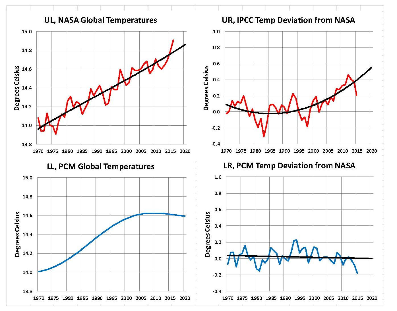
The first plot, UL is a plot of the NASA temperature anomaly converted to degrees Celsius and shown in red with a black trend line added. There has been a very clear reversal in the upward movement of global temperatures since about 2001 and neither the UN IPCC nor anyone else has an explanation for this 13 years later. Since CO2 has continued to increase at what could be argued an increasing rate, this raises serious doubts about the logic programmed into all the IPCC global climate models.
The next plot UR, also in red, shows the IPCC estimates of what the Global temperature should be, based on Hansen’s Scenario B, with the NASA actual temperatures’ subtracted from them. Therefore this plot represents a deviation from what the Climate “believers” KNOW what the temperature should be; with a positive value indicating the IPCC values are higher than actual and a negative value indicating the IPCC values are lower than actual, as measured by NASA. A black trend line is added and we can clearly see that the deviation from expected is increasing at an increasing rate. This makes sense since the IPCC models project increased temperatures based primarily on the increasing level of CO2 in the earth’s atmosphere. Unfortunately, for them, the actual temperatures from NASA are trending down (even as they try to hide the down ward movement with data manipulation) since other factors are in play, therefore each year the gap between them widens. Since we have 13 years of observations’ showing this pattern it becomes hard to justify a continuing belief in the IPCC climate models, there is obviously something very wrong here.
The next plot LL shown in blue is based on the equations in the PCM climate model described in previous papers and posts here and since it is generated by “equations” a trend line is not needed. As can be seen the PCM, LL, there is a 69.1 year cycle that moves the trend line up and then down a total of 0.29O Celsius and we are now in the downward portion of that trend (-.01491O C per year) which will continue until around 2035. This short cycle is clearly observed in the raw NASA data in the LOTI table going back to 1868. Then there is a long trend, 1036.7 years with an up and down of 1.65O Celsius (.00396O C per year) also observed in the NASA data. Lastly, there is CO2 adding about .007O Celsius per year so they basically wash out at -.0039 O C per year, which matches the current holding pattern we are experiencing. After about 2035 the short cycle will have bottomed and turn up and all three will be on the upswing again. These are all round numbers shown here as representative values.
The last plot LR in blue uses the same logic as used in the UR plot, here we use the PCM estimates of what the Global temperature should be with the NASA actual temperatures’ subtracted from them. A positive value indicates the PCM values are higher than actual and a negative value indicates the PCM values are lower than expected. A black trend line was added and it clearly shows that the PCM model is tracking the NASA actual values very closely. In, fact since 1970 the PCM model has rarely been off by more than +/- 0.1 degrees Celsius until the last few months where the manipulation showed up and has an average trend of almost zero error, while the IPCC models are erratic and are were approaching an error rate of over +0.4O C above expected until the last few months.
Note: Since I first started posting this monthly analysis a year and a half ago NOAA and NASA were directed make the global temperatures fit the political narrative that the planet was over heating and something drastic need to be done right now. The problem was as shown in this analysis the “real” world temperatures were not at the level that the IPCC GCM’s said they should be. Major adjustments to the data have been made that give the illusion that temperatures are going up even though they are not. However, as this analysis shows even with the manipulation that has destroyed all credibility from NOAA and NASA they cannot get the global temperatures even close to what their false theory claims they should be.
The next Chart shows the PCM model and all the various government plots related to climate change from 1875 through 2075. Clearly within the next dozen years we will know one way or the other which kind of climate model works. One based on observations and the other based on questionable science. There is no disrespect meant against the real climate scientists that have been marginalized this disrespect is meant for the political scientists who are the worst kind as they work for money not for the truth. Unfortunately, over the past year NASA has been directed by the current administration to make the global temperature match what the IPCC climate models predict it should be; therefore we see the very odd plot in the oval in the following Chart.
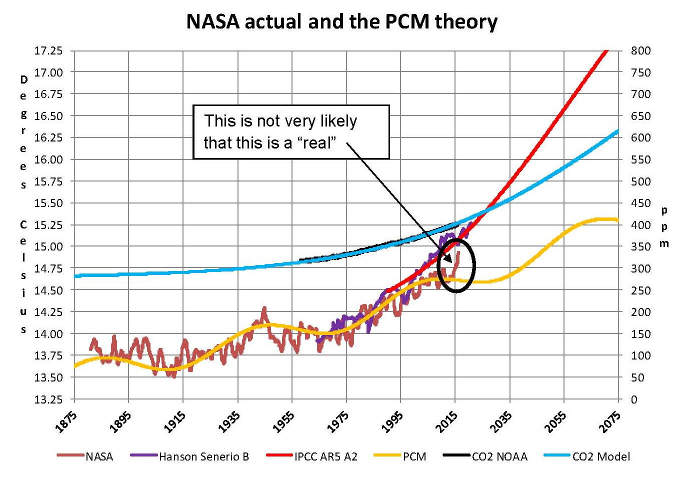
In summary, the IPCC models were designed before a true picture of the world’s climate was understood. During the 1980’s and 1990’s CO2 levels were going up and the world temperature was also going up so there appeared to be correlation and causation. The mistake that was made was looking at only a ~20 year period when the real variations in climate move in much longer cycles. Those other cycles can be observed in the NASA data but they were ignored for some reason. By ignoring those trends and focusing only on CO2 the models will be unable to correctly plot global temperatures until they are fixed.
Lastly, the next chart shows what a plot of the PCM model, in yellow, would look like from the year 1400 to the year 2900. The plot matches reasonably well with history and fits the current NASA-GISS table LOTI data, in red, very closely, despite homogenization. I understand that this model is not based on physics but it is also not curve fitting. It’s based on observed reoccurring patterns in the climate. These patterns can be modeled and when they are, you get a plot that works better than any of the IPCC’s GCM’s. If the conditions that create these patterns do not change and CO2 continues to increase to 800 ppm or even 1000 ppm than this model will work into the foreseeable future. 150 years from now global temperatures will peak at around 15.75 to 16.00 degrees C and then will be on the downside of the long cycle for the next 500 years. The overall effect of CO2 reaching levels of 1000 ppm or even higher will be about 1.5 degrees C which is about the same as that of the long cycle. The Green plot shows the pattern with no change in CO2 from the pre-industrial era of ~280 ppm.
Carbon Dioxide is not capable of doing what Hansen and Gore claim!
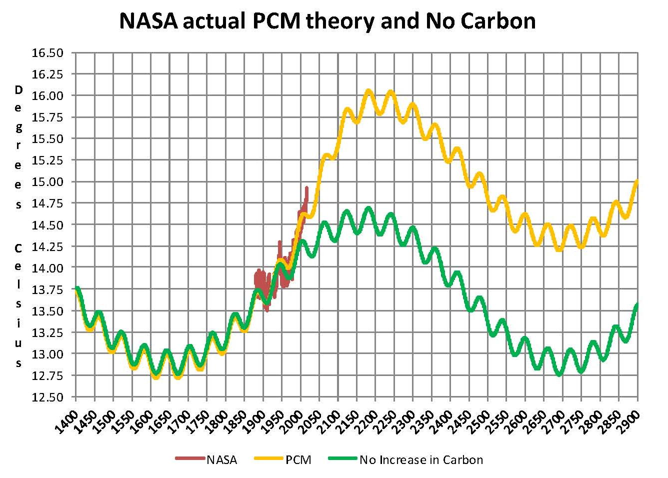
The purpose of this post is to make people aware of the errors inherent in the IPCC models so that they can be corrected.
The Obama administration’s “need” for a binding UN climate treaty with mandated CO2 reductions in Europe and America was achieved as predicted at the COP12 conference in Paris in December 2015. To support this endeavor NASA was forced to show ever increasing global temperatures that will make less and less sense based on observations and satellite data which will all be dismissed or ignored. Within a few years the manipulation will be obvious even to those without knowledge in the subject.
Sir Karl Raimund Popper (28 July 1902 – 17 September 1994) was an Austrian and British philosopher and a professor at the London School of Economics. He is considered one of the most influential philosophers for science of the 20th century, and he also wrote extensively on social and political philosophy. The following quotes of his apply to this subject.
If we are uncritical we shall always find what we want: we shall look for, and find, confirmations, and we shall look away from, and not see, whatever might be dangerous to our pet theories.
Whenever a theory appears to you as the only possible one, take this as a sign that you have neither understood the theory nor the problem which it was intended to solve.
… (S)cience is one of the very few human activities — perhaps the only one — in which errors are systematically criticized and fairly often, in time, corrected.
I have created this site to help people have fun in the kitchen. I write about enjoying life both in and out of my kitchen. Life is short! Make the most of it and enjoy!
De Oppresso Liber
A group of Americans united by our commitment to Freedom, Constitutional Governance, and Civic Duty.
Share the truth at whatever cost.
De Oppresso Liber
Uncensored updates on world events, economics, the environment and medicine
De Oppresso Liber
This is a library of News Events not reported by the Main Stream Media documenting & connecting the dots on How the Obama Marxist Liberal agenda is destroying America
Australia's Front Line | Since 2011
See what War is like and how it affects our Warriors
Nwo News, End Time, Deep State, World News, No Fake News
De Oppresso Liber
Politics | Talk | Opinion - Contact Info: stellasplace@wowway.com
Exposition and Encouragement
The Physician Wellness Movement and Illegitimate Authority: The Need for Revolt and Reconstruction
Real Estate Lending
