
“The world has less than a decade to change course to avoid irreversible ecological catastrophe, the UN warned today.” The Guardian Nov 28 2007
“It’s tough to make predictions, especially about the future.” Yogi Berra
Introduction
Global extinction due to global warming has been predicted more times than climate activist, Leo DiCaprio, has traveled by private jet. But where do these predictions come from? If you thought it was just calculated from the simple, well known relationship between CO2 and solar energy spectrum absorption, you would only expect to see about 0.5o C increase from pre-industrial temperatures as a result of CO2 doubling, due to the logarithmic nature of the relationship.
 Figure 1: Incremental warming effect of CO2 alone [1]
The runaway 3-6o C and higher temperature increase model predictions depend on coupled feedbacks from many other factors, including water vapour (the most important greenhouse gas), albedo (the proportion of energy reflected from the surface – e.g. more/less ice or clouds, more/less reflection) and aerosols, just to mention a few, which theoretically may amplify the small incremental CO2 heating effect. Because of the complexity of these interrelationships, the only way to make predictions is with climate models because they can’t be directly calculated.
The purpose of this article is to explain to the non-expert, how climate models work, rather than a focus on the issues underlying the actual climate science, since the models are the primary ‘evidence’ used by those claiming a climate crisis. The first problem, of course, is no model forecast is evidence of anything. It’s just a forecast, so it’s important to understand how the forecasts are made, the assumptions behind them and their reliability.
How do Climate Models Work?
In order to represent the earth in a computer model, a grid of cells is constructed from the bottom of the ocean to the top of the atmosphere. Within each cell, the component properties, such as temperature, pressure, solids, liquids and vapour, are uniform.
The size of the cells varies between models and within models. Ideally, they should be as small as possible as properties vary continuously in the real world, but the resolution is constrained by computing power. Typically, the cell area is around 100×100 km2 even though there is considerable atmospheric variation over such distances, requiring each of the physical properties within the cell to be averaged to a single value. This introduces an unavoidable error into the models even before they start to run.
The number of cells in a model varies, but the typical order of magnitude is around 2 million.
 Figure 2: Typical grid used in climate models [2]
Once the grid has been constructed, the component properties of each these cells must be determined. There aren’t, of course, 2 million data stations in the atmosphere and ocean. The current number of data points is around 10,000 (ground weather stations, balloons and ocean buoys), plus we have satellite data since 1978, but historically the coverage is poor. As a result, when initialising a climate model starting 150 years ago, there is almost no data available for most of the land surface, poles and oceans, and nothing above the surface or in the ocean depths. This should be understood to be a major concern.
 Figure 3: Global weather stations circa 1885 [3]
Once initialised, the model goes through a series of timesteps. At each step, for each cell, the properties of the adjacent cells are compared. If one such cell is at a higher pressure, fluid will flow from that cell to the next. If it is at higher temperature, it warms the next cell (whilst cooling itself). This might cause ice to melt or water to evaporate, but evaporation has a cooling effect. If polar ice melts, there is less energy reflected that causes further heating. Aerosols in the cell can result in heating or cooling and an increase or decrease in precipitation, depending on the type.
Increased precipitation can increase plant growth as does increased CO2. This will change the albedo of the surface as well as the humidity. Higher temperatures cause greater evaporation from oceans which cools the oceans and increases cloud cover. Climate models can’t model clouds due to the low resolution of the grid, and whether clouds increase surface temperature or reduce it, depends on the type of cloud.
It’s complicated! Of course, this all happens in 3 dimensions and to every cell resulting in considerable feedback to be calculated at each timestep.
The timesteps can be as short as half an hour. Remember, the terminator, the point at which day turns into night, travels across the earth’s surface at about 1700 km/hr at the equator, so even half hourly timesteps introduce further error into the calculation, but again, computing power is a constraint.
While the changes in temperatures and pressures between cells are calculated according to the laws of thermodynamics and fluid mechanics, many other changes aren’t calculated. They rely on parameterisation. For example, the albedo forcing varies from icecaps to Amazon jungle to Sahara desert to oceans to cloud cover and all the reflectivity types in between. These properties are just assigned and their impacts on other properties are determined from lookup tables, not calculated. Parameterisation is also used for cloud and aerosol impacts on temperature and precipitation. Any important factor that occurs on a subgrid scale, such as storms and ocean eddy currents must also be parameterised with an averaged impact used for the whole grid cell. Whilst the effects of these factors are based on observations, the parameterisation is far more a qualitative rather than a quantitative process, and often described by modelers themselves as an art, that introduces further error. Direct measurement of these effects and how they are coupled to other factors is extremely difficult and poorly understood.
Within the atmosphere in particular, there can be sharp boundary layers that cause the models to crash. These sharp variations have to be smoothed.
Energy transfers between atmosphere and ocean are also problematic. The most energetic heat transfers occur at subgrid scales that must be averaged over much larger areas.
Cloud formation depends on processes at the millimeter level and are just impossible to model. Clouds can both warm as well as cool. Any warming increases evaporation (that cools the surface) resulting in an increase in cloud particulates. Aerosols also affect cloud formation at a micro level. All these effects must be averaged in the models.
When the grid approximations are combined with every timestep, further errors are introduced and with half hour timesteps over 150 years, that’s over 2.6 million timesteps! Unfortunately, these errors aren’t self-correcting. Instead this numerical dispersion accumulates over the model run, but there is a technique that climate modelers use to overcome this, which I describe shortly.
 Figure 4: How grid cells interact with adjacent cells [4]
Model Initialisation
After the construction of any type of computer model, there is an initalisation process whereby the model is checked to see whether the starting values in each of the cells are physically consistent with one another. For example, if you are modelling a bridge to see whether the design will withstand high winds and earthquakes, you make sure that before you impose any external forces onto the model structure other than gravity, that it meets all the expected stresses and strains of a static structure. Afterall, if the initial conditions of your model are incorrect, how can you rely on it to predict what will happen when external forces are imposed in the model?
Fortunately, for most computer models, the properties of the components are quite well known and the initial condition is static, the only external force being gravity. If your bridge doesn’t stay up on initialisation, there is something seriously wrong with either your model or design!
With climate models, we have two problems with initialisation. Firstly, as previously mentioned, we have very little data for time zero, whenever we chose that to be. Secondly, at time zero, the model is not in a static steady state as is the case for pretty much every other computer model that has been developed. At time zero, there could be a blizzard in Siberia, a typhoon in Japan, monsoons in Mumbai and a heatwave in southern Australia, not to mention the odd volcanic explosion, which could all be gone in a day or so.
There is never a steady state point in time for the climate, so it’s impossible to validate climate models on initialisation.
The best climate modelers can hope for is that their bright shiny new model doesn’t crash in the first few timesteps.
The climate system is chaotic which essentially means any model will be a poor predictor of the future – you can’t even make a model of a lottery ball machine (which is a comparatively a much simpler and smaller interacting system) and use it to predict the outcome of the next draw.
So, if climate models are populated with little more than educated guesses instead of actual observational data at time zero, and errors accumulate with every timestep, how do climate modelers address this problem?
History matching
If the system that’s being computer modelled has been in operation for some time, you can use that data to tune the model and then start the forecast before that period finishes to see how well it matches before making predictions. Unlike other computer modelers, climate modelers call this ‘hindcasting’ because it doesn’t sound like they are manipulating the model parameters to fit the data.
The theory is, that even though climate model construction has many flaws, such as large grid sizes, patchy data of dubious quality in the early years, and poorly understood physical phenomena driving the climate that has been parameterised, that you can tune the model during hindcasting within parameter uncertainties to overcome all these deficiencies.
While it’s true that you can tune the model to get a reasonable match with at least some components of history, the match isn’t unique.
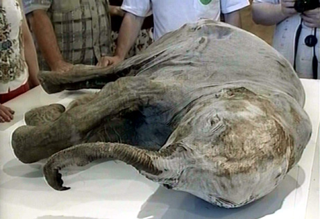
When computer models were first being used last century, the famous mathematician, John Von Neumann, said:
“with four parameters I can fit an elephant, with five I can make him wiggle his trunk”
In climate models there are hundreds of parameters that can be tuned to match history. What this means is there is an almost infinite number of ways to achieve a match. Yes, many of these are non-physical and are discarded, but there is no unique solution as the uncertainty on many of the parameters is large and as long as you tune within the uncertainty limits, innumerable matches can still be found.
An additional flaw in the history matching process is the length of some of the natural cycles. For example, ocean circulation takes place over hundreds of years, and we don’t even have 100 years of data with which to match it.
In addition, it’s difficult to history match to all climate variables. While global average surface temperature is the primary objective of the history matching process, other data, such a tropospheric temperatures, regional temperatures and precipitation, diurnal minimums and maximums are poorly matched.
Even so, can the history matching of the primary variable, average global surface temperature, constrain the accumulating errors that inevitably occur with each model timestep?
Forecasting
Consider a shotgun. When the trigger is pulled, the pellets from the cartridge travel down the barrel, but there is also lateral movement of the pellets. The purpose of the shotgun barrel is to dampen the lateral movements and to narrow the spread when the pellets leave the barrel. It’s well known that shotguns have limited accuracy over long distances and there will be a shot pattern that grows with distance. The history match period for a climate model is like the barrel of the shotgun. So what happens when the model moves from matching to forecasting mode?
 Figure 5: IPCC models in forecast mode for the Mid-Troposphere vs Balloon and Satellite observations [5]
Like the shotgun pellets leaving the barrel, numerical dispersion takes over in the forecasting phase. Each of the 73 models in Figure 5 has been history matched, but outside the constraints of the matching period, they quickly diverge.
Now at most only one of these models can be correct, but more likely, none of them are. If this was a real scientific process, the hottest two thirds of the models would be rejected by the International Panel for Climate Change (IPCC), and further study focused on the models closest to the observations. But they don’t do that for a number of reasons.
Firstly, if they reject most of the models, there would be outrage amongst the climate scientist community, especially from the rejected teams due to their subsequent loss of funding. More importantly, the so called 97% consensus would instantly evaporate.
Secondly, once the hottest models were rejected, the forecast for 2100 would be about 1.5o C increase (due predominately to natural warming) and there would be no panic, and the gravy train would end.
So how should the IPPC reconcile this wide range of forecasts?
Imagine you wanted to know the value of bitcoin 10 years from now so you can make an investment decision today. You could consult an economist, but we all know how useless their predictions are. So instead, you consult an astrologer, but you worry whether you should bet all your money on a single prediction. Just to be safe, you consult 100 astrologers, but they give you a very wide range of predictions. Well, what should you do now? You could do what the IPCC does, and just average all the predictions.
You can’t improve the accuracy of garbage by averaging it.
An Alternative Approach
Climate modelers claim that a history match isn’t possible without including CO2 forcing. This is may be true using the approach described here with its many approximations, and only tuning the model to a single benchmark (surface temperature) and ignoring deviations from others (such as tropospheric temperature), but analytic (as opposed to numeric) models have achieved matches without CO2 forcing. These are models, based purely on historic climate cycles that identify the harmonics using a mathematical technique of signal analysis, which deconstructs long and short term natural cycles of different periods and amplitudes without considering changes in CO2 concentration.
In Figure 6, a comparison is made between the IPCC predictions and a prediction from just one analytic harmonic model that doesn’t depend on CO2 warming. A match to history can be achieved through harmonic analysis and provides a much more conservative prediction that correctly forecasts the current pause in temperature increase, unlike the IPCC models. The purpose of this example isn’t to claim that this model is more accurate, it’s just another model, but to dispel the myth that there is no way history can be explained without anthropogenic CO2 forcing and to show that it’s possible to explain the changes in temperature with natural variation as the predominant driver.
 Figure 6: Comparison of the IPCC model predictions with those from a harmonic analytical model [6]
In summary:
Climate models can’t be validated on initiatialisation due to lack of data and a chaotic initial state.
Model resolutions are too low to represent many climate factors.
Many of the forcing factors are parameterised as they can’t be calculated by the models.
Uncertainties in the parameterisation process mean that there is no unique solution to the history matching.
Numerical dispersion beyond the history matching phase results in a large divergence in the models.
The IPCC refuses to discard models that don’t match the observed data in the prediction phase – which is almost all of them.
The question now is, do you have the confidence to invest trillions of dollars and reduce standards of living for billions of people, to stop climate model predicted global warming or should we just adapt to the natural changes as we always have?
Greg Chapman is a former (non-climate) computer modeler.
Footnotes
[1] https://www.adividedworld.com/scientific-issues/thermodynamic-effects-of-atmospheric-carbon-dioxide-revisited/
[2] https://serc.carleton.edu/eet/envisioningclimatechange/part_2.html
[3] https://climateaudit.org/2008/02/10/historical-station-distribution/
[4] http://www.atmo.arizona.edu/students/courselinks/fall16/atmo336/lectures/sec6/weather_forecast.html
[5] https://www.drroyspencer.com/2013/06/still-epic-fail-73-climate-models-vs-measurements-running-5-year-means/
Whilst climate models are tuned to surface temperatures, they predict a tropospheric hotspot that doesn’t exist. This on its own should invalidate the models.
[6] https://wattsupwiththat.com/2012/01/09/scaffeta-on-his-latest-paper-harmonic-climate-model-versus-the-ipcc-general-circulation-climate-models/


