The Blackbody Temperature of the Planet Earth


This is a key step in the Climate Debate

Determining the ‘exact’ Blackbody temperature of the planet is the first step in determining what the “greenhouse’ effect is; for without that value all else is either speculation or based on an unreliable value. This leads us to a quandary since the plant is a global spinning around a titled axis and with an elliptical orbit around the sun Figure 1 which is the source of virtually all the energy that heats the planet. Clearly with these facts there cannot be one temperature for the planet and so an average can be very misleading and lead to false conclusions.

Traditional calculations of the planets black body temperature ignore the variables which then lead one to assume a steady state situation verses the real dynamic situation that drives climate. To justify this assumption a general statement that the variances are too small to have any meaningful effect are promoted. I some cases with fewer variables this might be true but in this case I think not.

These are the main Variables:

1. The sun has a cycle of about eleven years and that gives a small variation in the suns output of about 1%
2. The planet has an elliptical Orbit that varies by 3.34% or 4,999,849 miles
3. The axial tilt of the planet is 23.4 degrees which causes winter and summer to alternate between Aphelion and Perihelion about every 10,000 years
4. The planet is a sphere so only one side faces the sun at any given moment
5. The sun’s energy reaches the planet on a line drawn from the center of the sun to the center of the planet which only intersects the equator twice a year
6. The energy from the sun is concentrated around this line
7. The planet is a sphere so the suns radiation drops off in all directions from this line by a Cosine factor to zero at the edge 90 degrees from the center line
8. The spin and tilt of the planet means that the center line moves up 23.4 degrees and down 23.4 degrees during the course of one orbit
9. That movement means the distribution of energy also moves
10. The distribution of land and ocean are not uniform on the planet
11. The albedo of the planet is a variable not a constant
12. Energy from the core adds a small amount of energy
13. Tidal forces from the sun and the moon also add some energy
14. Energy is carried North and South from the hot spot centered on the line by the atmosphere and the ocean
15. The Coriolis Effect along with tidal forces drive thermal transfer north and south at an angle and these are then main contributors to the climate

FIGURE 01
Figure 1, the Earth’s orbit

FIGURE 02
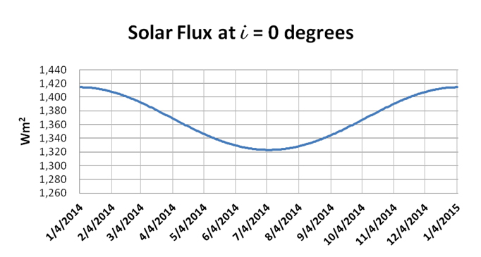
Figure 2, orbital changes in solar flux

There are three sources of energy that determine the climate on the earth: the radiation from the sun which is said to be 1366 Wm2 The actual value based on the orbital range is from 1414.4 Wm2 in January to 1323.0 Wm2 in July Figure 2 and there is also an eleven year sun spot cycle with a range of 1.37 Wm2. The hot core of the planet adds ~0.087 W/m2 and the gravitational effects of the moon and the sun (tides) adds another ~.00738 Wm2. Of these three the sun’s radiation is by far the most important but considering all three the range during an eleven year solar cycle is from a high of ~1415.3 Wm2 to a low of ~1322.4 Wm2 so a more accurate mean would be 1368.34 Wm2.

The energy emitted by the planet must equal the energy absorbed by the planet and we can calculate this using the Stefan-Boltzmann Law. Which is the energy flux emitted by a blackbody is related to the fourth power of the body’s absolute temperature. The tidal and core temperatures are added after the albedo adjustment.

E = σT4
σ = 5.67×10⁻⁸ Wm2 K sec
A = 30.6% (the planets albedo, this is not a constant)

σTbb4 x (4πRe2) = S πRe2 x (1-A)
σTbb4 = S/4 * (1-A)
σTbb4 = 1368.24/4 Wm2 * (1-A)
σTbb4 = 342.16 Wm2 * (1-A)
σTbb4 = 254.36 Wm2

Earth’s Blackbody temperature                      Earth’s surface temperature

Tbb = 252.23O K (-20.92O C) low                  Ts = ~287.75O K (14.6 O C) today
Tbb = 254.36O K (-18.79O C) mean
Tbb = 256.54O K (-16.51O C) high

The difference between the Blackbody and the current temperatures is what we call the ‘greenhouse’ effect that averages 33.36O Celsius (C), today, although the range is from 35.52O C to 31.11O C from variations in the 11 year solar cycle. Despite this variation in incoming solar flux the planet’s temperatures is very stable. Other factors are also important in doing climate work such as the solar energy is concentrated between about +/- 30 degrees of the equator maybe a bit more. And the heat from the core and probably the tides is concentrated where the crust is the thinnest under the oceans and this concentration of energy core heat and tides) combined with Coriolis forces is probably what drives the ocean currents. In my opinion these other important factors are not being considered properly in the climate models.

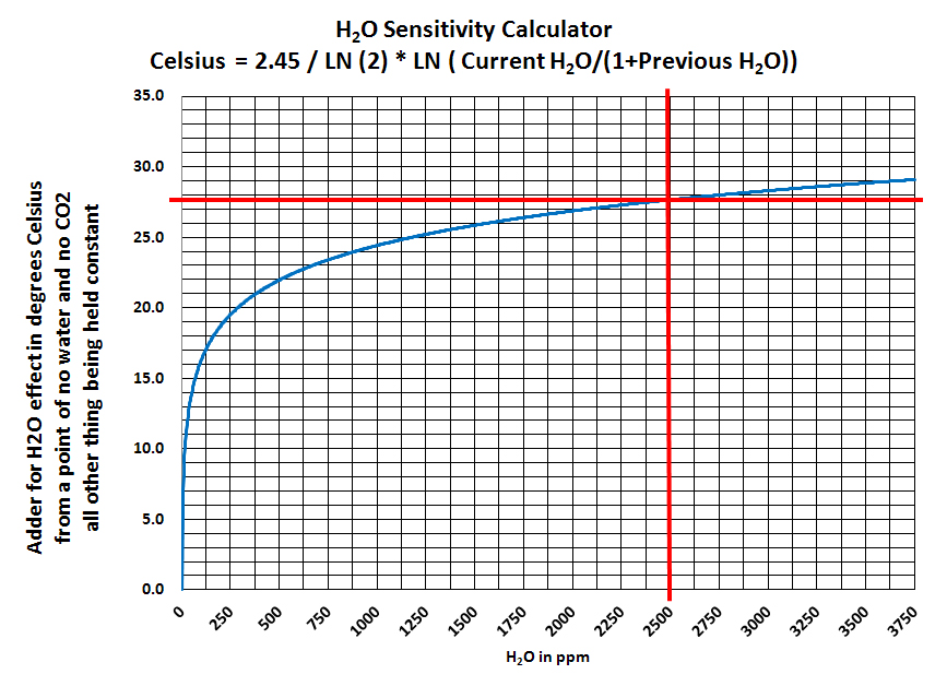
We also know from geological studies Figure 3 that the planets temperature has been relatively stable over the past 600 million years with a mean of about 17O C or 290O Kelvin (K) and with a range of plus or minus 5O K or C based on the information in Figure 3. During the past 250 million years CO2 concentrations have ranged from a low of ~280 ppm (a historic low)in 1800 to the present low of 400 ppm to a high of over 2,000 ppm probably averaging around 1,500 ppm. There was only one other period in the past 600 million years with CO2 this low. Going back further CO2 was estimated to be as high is 7000 ppm, but we will ignore that for now.

This means that whatever the processes are that relate to determining the thermal balance of the planet they must work within this range to be valid. Although Figure 3 shows a range of 10O C it would be prudent to spend resources to determine these values with as great accuracy as possible. We’ll assume a mean of 16O C with a range from 10O to 22O C as being more reasonable. Also we are now in one of only three cold periods which are very rare in the past 600 million years and if we count that partial dip 150 million years ago that means that there is probably a 150 million year cycle there; maybe one of those first determined my Milutin Milankovic.

FIGURE 03
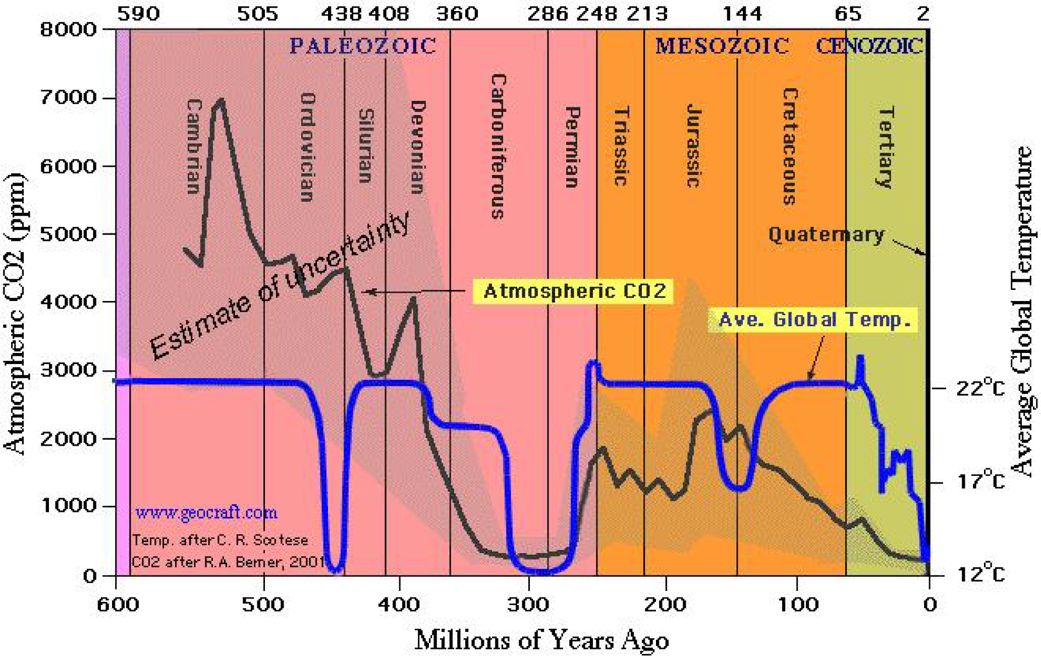
Figure 3, Geological temperatures and Carbon Dioxide

Additional discussion as to the so called “greenhouse” effect must start with the important correction that this process is not a true greenhouse effect, since it is not the same process that occurs in a greenhouse used to grow food. The actual process that occurs is based on the structure of the atoms involved and how they interact with the various frequencies of visible and infrared radiation that are in play on the planet. However at this point in time there is no way to correct for the misuse of the words so we are stuck with it and all the complications that therefore arise in trying to properly discuss the issue with lay people and even some with technical knowledge.

The greenhouse effect occurs within the earth’s atmosphere and the main constitutes of wet air, by volume ppmv (parts per million by volume) are listed in the following table. Water vapor is 0.25% over the full atmosphere but locally it can be 0.001% to 5% depending on local conditions. Water and CO2 are mostly near the surface not in the upper atmosphere so the bulk of the greenhouse effect must be close to the surface.

                                   Gas Volume Percentage
Nitrogen (N2)                                 780,840 ppmv   78.8842%
Oxygen (O2)                                   209,460 ppmv   20.8924%
Argon (Ar)                                          9,340 ppmv    0.9316%
Water vapor (H2O)                             2,500 ppmv     0.2494%
Carbon dioxide (CO2)                            400 ppmv     0.0399%
Neon (Ne)                                          18.18 ppmv     0.001813%
Helium (He)                                         5.24 ppmv     0.000523%
Methane (CH4)                                    1.79 ppmv      0.000179%

There are only two of these gases that are relevant to determining how that 33O C (today) happens. That is not to say the others do not contribute but that at the present concentrations of Water H2O and Carbon Dioxide CO2 they are the main determinants. And since we know the range of temperatures that have existed geologically then we have set the range which these to gases must interact in, meaning that any set of equations or models or theories that predict values outside this range must be suspect based on geological evidence.

Also it must be kept in mind that the solar flux falls on a spot centered on a line drawn from the center of the earth to the center of the sun and because of the 23.5O axial tilt of the planet this “Hot” spot moves up and down as the planet moves though its orbit. Because of the shape of the planet the intensity falls off quickly as we move north and south and east and west according to a cosine factor so the heat energy is mostly over oceans near the equator where the atmosphere is the densest.

The first image below Figure 4 shows a recent distribution of water across the planet and it is clearly concentrated over the oceans close to the equator and that results in the heat imbalance and therefore movement north and south as shown in the second image Figure 5.

FIGURE 04
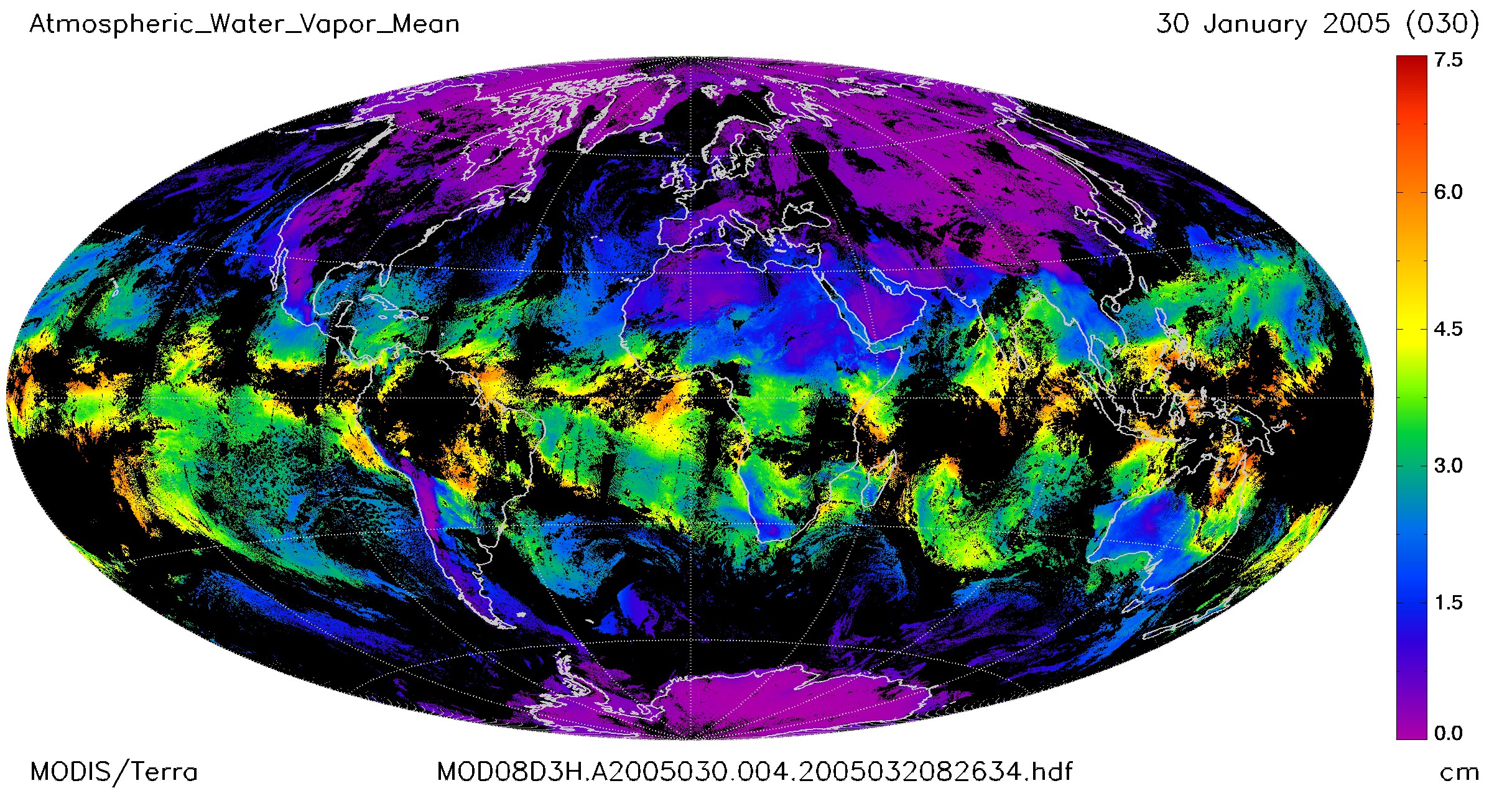
Figure 4, water vapor concentrated near the equator

FIGURE 05
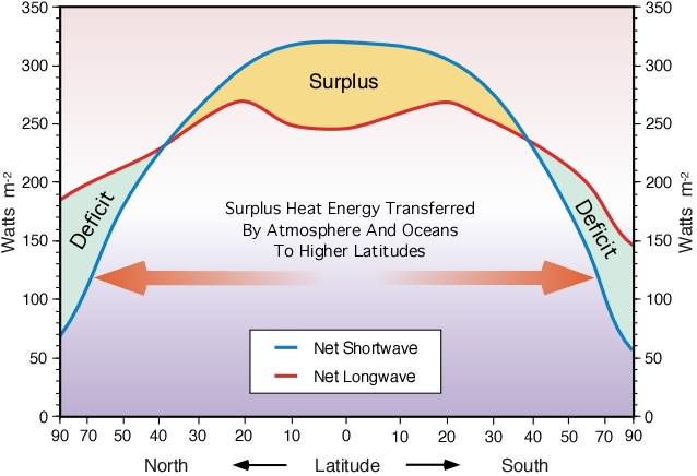
Figure 5, basic heat flows from the equator north and south

The next two images show how that energy is moved by the water Figure 6 and the atmosphere north and south from the equator Figure 7.

FIGURE 06
Figure 6, Ocean currents

FIGURE 07
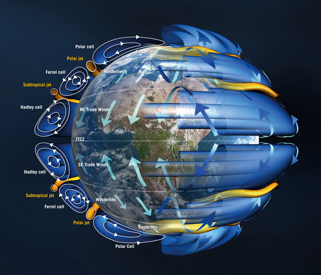
Figure 7, Atmospheric heat flows

In summary we now know that the Blackbody temperature of the planet is a variable.

Tbbl   = 252.23O K (-20.92O C) low at Aphelion
Tbbm = 254.36O K (-18.79O C) and the yearly mean
Tbbh  = 256.54O K (-16.51O C) high at Perihelion

Therefore the ‘greenhouse effect must also be a variable.

Ts = ~287.75O K (14.6O C) today

Ghl =   Tbbl + Ts    = 35.52O C
Ghm = Tbbm + Ts = 32.39O C
Ghh =  Tbbh + Ts   = 31.11O C

The range in temperature just from orbital changes is therefore 4.41 O C which is significantly more than the warming that the IPCC claims has happened. These are hard numbers based on the solar flux which is known and the orbital parameters of the Earth that are also known. The large variances come from the Stefan-Boltzmann Law; which is the energy flux emitted by a Blackbody is related to the fourth power of the body’s absolute temperature. The fourth power in the equation magnifies the small variation in solar flux significantly.

The Real Job’s Report for June 2014


How many jobs were created since 2007 not last month

Based on the BLS July 3, 2014 Release USDL-14-1243 we have the following analysis using the numbers shown in Table B-1 and A-8. Then we use a DOD monthly report for Active duty military to add to the other two of 1.36 million soldiers. By doing this we get a more complete picture of those that are getting pay for some form of work and are therefore not on public assistance or retired. For reference that report claims that 288,000 jobs were created in June.

The first thing that came out when we look at what has happened since the high point of the previous growth period in October 2007 was that we are still short 394,630 jobs from then making this the slowest recovery on record. But there were categories of gains and categories of loss’s so what are they?

JOBS June 2014

The total gains and losses for all the other categories give a net gain of 428,990 which when combined with the two table’s leaves us with a net loss of jobs since October 2007 of -394,630. But we also see that close to half of the gaining categories are low paying jobs and that most all the losing categories were good paying jobs. It would therefore appear that not only are there fewer jobs but there has been a shift out of traditional middle class jobs to lower paying personal service jobs in food service nursing homes and the like. Without seeing the income distributions that is speculation but the categories speak for themselves.

The only real winners in the past 7 years appear to be the upper middle class and the upper class as those categories of government workers, financial advisers, legal and doctors have increased.

Obama’s Transformation is almost completed


But the results will not be what he expected

The American government has been infiltrated by the Muslin brotherhood which was formed in Egypt decades ago and this has created a major conflict. The Brotherhood are Sunni Muslims who are 80% of the Muslims and they have no love for the Shea Muslims who are less than 20% of the Muslims. The conflict that arises is that Iran is predominantly Shea and the Saudis and the ISIS are Sunni; and the more fundamental Muslims e.g. the ISIS want to reestablish a Caliphate which rules using Sharia Law. The problems that the Muslims have and therefore this administration has is that Sharia Law is basically what existed in the Arabian peninsula when Mohamed started the Islamic beliefs which made the then existing tribal habits customs or laws of the 7th century inhabitants of that part of the world into unchangeable religious dogma. Sharia Law is TOTALLY INCOMPATIBLE with Western Civilization and that is indisputable fact that even the American founding fathers including the Progressives favorite, Thomas Jefferson understood.

When Obama and his Progressive/Marxist followers started the policies of Fundamental Transformation of America they also believed that this transformation could be spread worldwide and since their handlers in the Muslim Brotherhood supported this view the Arab Spring was initiated. The Brotherhood wanted the existing leaders removed since they were not true believers in the new Caliphate that they wanted. I would not be surprised to learn that they also had an influence in the Bush administration for the 2003 invasion to topple Saddam Hussein; although I do not belief that Bush had anything but the best interests for America as he was not looking to Fundamentally Transform the country.

Off the subject but relevant is that the Cloward-Piven strategy is what Obama is using to change the country and it is, to first cause a breakdown of the society that you want to change by using it against itself. It this case to use environmental and social policies to destroy the middle class by making it to easy to not work and by putting so many regulations in place that the small business go under. I drive a lot in Cleveland and I see hundreds of abandoned buildings and store fronts in all parts of the city.

Because of the way the Bureau of Labor Statistics (BLS) reports their numbers many if not most of those closing business to not show in the official monthly numbers; this segment has taken a large hit since 2007 and has not recovered. Neither has the good production section recovered and again a large percentage of the middle class was employed there. There are now (4,625,800) fewer people earning a living today in good paying jobs then in 2007 and the 3,816,400 increase in mostly lower paying jobs leaves a net loss of over (809,440) jobs.

To achieve this reduction in jobs the federal government, not counting the Post Office, has been increased by 8.6% or 168,300 jobs presumably these are mostly in Washington DC and are good paying jobs. So one could say that for every federal job created we lost almost 5 private sector jobs, and the transformation is not over.

As the middle class jobs are eliminated more goods have to be produced in China, India and else ware to make up the difference and that means more borrowing from those countries to pay for those goods and services. Since October 2007 $3,892,702,000,000 has been borrowed from these countries and when added to domestic borrowing the total borrowed is $8,437,873,000,000 more debt since then.

So one could say that to get rid of one good paying job we had to borrow $10,424,334 a good return for someone but not the middle class.

The reduction in jobs and the increase in debt is a direct result of the policies of those running the government as they try to move us from a market based system to a central planning based system. There are many of us that don’t think that will turn out well but the voters have spoken and this is therefore either what they want or they have partaken of the Kool Aid.

It cannot be dismissed that the Brotherhood may have contributed to this transformation but whether it was or not the transformation has been done and the result will be a diminished American economy and world presence; which leaves a power vacuum which must be filled to re-stabilize the world. The last time this happened was in the 1920-1930’s and that resulted in WW II. If one wants to look at patterns one would say that a major war must happen and that the most likely date is 2018; and it will probably be with the Muslims’ since this administration has given them the opening that they need. The Brotherhoods influence in our government makes it impossible to counter this infiltration without being accused of being anti-Muslim so the deck has been dealt and the cards are all in the hands of the players and its only how they will be played that will determine the winner.

But we also know that the Obama administration is severely deficient in the quality of the strategic thinking ability of its members so it’s very unlikely they can play their cards to a good outcome ….

The Collapse of the US Economic System


NO JOBS

The Great Recession actually started in November 2007 as that was the month that jobs in the US started to decline from their peak in the previous month October. The collapse in the financial markets started 12 months later in October 2008 just prior to the presidential election. This analysis is intended to show what was in place at the peak October 2007 compared to today May 2014. In this analysis we will use only official government data; however it will be adjusted to reflect TOTAL Employment not just what the Bureau of Labor Statistics (BLS) shows each month with their employment status report. They don’t report the farmers, the self-employed and the military; although those numbers are available, so we just add them to the BLS numbers to get a truer picture of “all” the people earning a living.

All these numbers can be found on the BLS website the most current is USDL-14-0987

For the peak October 2007, the population of the country was 301,811,120 and the BLS showed in their Table B-1 that there were 138,361,400 working comprising 50.04% of the populations in the following three major Categories:

Goods Producing            22,266,000     7.38%
Services                         93,767,500    31.07%
Government                   22,327,900     7.40%
TOTAL BLS                     138,361,400   45.84%

Next we add in the jobs the BLS doesn’t count.

Self Employed                  9,060,900     3.00%
Agriculture                       2,218,100       .73%
Military                             1,418,200       .47%
TOTAL                             12,697,200      4.20%

GRAND TOTAL               151,058,600     50.04%

For May 2014 53 months since the end of the recession the population of the country was 318,138,408 and the BLS showed in their Table B-1 that there were 138,462,300 working comprising 47.22% of the populations in the following three major Categories:

Goods Producing            19,009,000      5.98%
Services                          97,583,900    30.67%
Government                   21,869,400      6.87%
TOTAL                           138,462,300     43.52%

Next we add in the jobs the BLS doesn’t count.

Self Employed                  8,375,000      2.63%
Agriculture                       2,011,000        .63%
Military                             1,400,900        .44%
TOTAL                             11,786,900       3.70%

GRAND TOTAL               150,249,200     47.22%

The difference between the two periods is, by the BLS numbers, that we now have 100,900 more jobs than October 2007 which is good; however if we add back in the agriculture, self-employed and the military we are still short 809,440 jobs. This means there are 809,440 fewer people without a paycheck today than in November 2007. Also note that there are more people in the government than in the goods producing sectors in 2007 and and a lot more in 2014, that just doesn’t seem right.

Making this situation significantly worse are two other factors; the first being that the population has grown by 16,327,288 so that means that there are 16,327,288 more people to be support by 800,000 fewer workers. The second being that since the highest paying jobs for the middle class, in the good producing sectors, are down 3,257,000 jobs from October 2007 and the self employed are down another 685,900 for a total of 3,942,900 fewer middle class jobs. Offsetting this is an increase of 4,043,800 jobs (100,900 jobs more) but they are mostly in the lower paying job categories like food services and temporary help

So the bottom line is fewer people working and those that are working are bring home less money. The shift of a large portion of the manufacturing sector to China and India over the past dozen years has decimated the American middle class and swelled the rolls of those dependent of the federal government for various forms of transfer payments from food stamps to disability payments.

NO ECONOMIC OR POLITICAL SYSTEM CAN SUSTAIN THIS TRANSFORMATION BEING IMPOSED ON THE CITIZENS FROM THE PROGRESSIVE POLITICAL WINGS OF BOTH MAJOR PARTIES. THINGS WILL EITHER CHANGE OR THE AMERICAN SYSTEM WILL COLLAPSE.


Analysis of Global Temperature Trends, May 2014


What really going on with the Climate?

The analysis and plots shown here are based on the following: first NASA-GISS temperature anomalies (converted to degrees Celsius) as shown in their table LOTI, second James E. Hansen’s Scenario B data, which is the very core of the IPCC Global Climate models which was based on a CO2 sensitivity value of 3.0O Celsius, lastly, a plot based on an alternative climate model designated ‘PCM’ and based on a sensitively value of .65O Celsius. To smooth monthly variations a 12 month running average is used in all the plots. This information will be shown in four tables and updated each month as the new data comes in.

2014-May
The first plot, UL is a plot of the NASA temperature anomaly converted to degrees Celsius shown in red with a black trend line added. There has been a very clear reversal in the upward movement of global temperatures since about 2001 and neither the UN IPCC nor anyone else has an explanation for this. Since CO2 has continued to increase at what could be argued an increasing rate this raises serious doubts about the logic programmed into all the IPCC global climate models.

The next plot UR, also in red, shows the IPCC estimates of what the Global temperature should be, based on Hansen’s Scenario B, with the NASA actual temperatures’ subtracted from them. Therefore this plot represents a deviation from what the Climate “believers” KNOW what the temperature should be; with a positive value indicating the IPCC values are higher than actual and a negative value indicating the IPCC values are lower than actual. A black trend line is added and we can clearly see that the deviation from expected is increasing at an increasing rate. This makes sense since the IPCC models project increased temperatures based primarily on the increasing level of CO2 in the earth’s atmosphere. Unfortunately, for them, the actual temperatures from NASA are trending down (even as they try to hide the down ward movement with data manipulation) since other factors are in play, therefore each year the gap between them widens. Since we have 12 years of observations’ showing this pattern it becomes hard to justify a continuing belief in the IPCC climate models, there is obviously something very wrong.

The next plot LL shown in blue is based on the equations in the PCM climate model described in previous papers and posts here and since it is generated by “equations” a trend line is not needed. As can be seen the PCM, LL, and the NASA, UL, trend plots are very similar the reason being that in the PCM model there is a 68.2 year cycle that moves the trend line up and then down a total of .30O Celsius (currently negative .0070O Celsius per year); and we are now in the downward portion of that trend which will continue until around 2035. This short cycle is clearly observed in the raw NASA data in the LOTI table going back to 1880. Then there is the a long trend, 1052.6 years with an up and down of 1.36O Celsius (currently plus .0029O Celsius per year) also observed in the NASA data. Lastly there is CO2 adding about .005O Celsius per year so they messily wash out which matches the current holding pattern we are in. However with a few years the increasing downward trend of the short cycle will overpower the other tow and we will see drop of about .002O Celsius per year and that will be increasing until till around 2025. After about 2035 the short cycle will turn up and all three will be on the upswing again. These are all round numbers shown here are representative values.

The last plot LR in blue uses the same logic as used in the UR plot, here we use the PCM estimates of what the Global temperature should be with the NASA actual temperatures’ subtracted from them. A positive value indicates the PCM values are higher than actual and a negative value indicates the PCM values are lower than expected. A black trend line was added and it clearly shows that the PCM model is tracking the NASA actual values very closely. In, fact since 1970 the PCM model has rarely been off by more than +/- .1 degrees Celsius and has an average trend of almost zero error, while the IPCC models are erratic and are now approaching an error rate of +.5O above expected.

The IPCC models were designed before a true picture of the world’s climate was understood. During the 1980’s and 1990’s CO2levels were going up and the world temperature was also going up so there appeared to be correlation and causation. The mistake that was made was looking at only a 20 year period when the real variations in climate move in much longer cycles. Those other cycles can be observed in the NASA data but they were ignored for some reason. By ignoring those trends and focusing only on CO2 the models will be unable to correctly plot global temperatures until they are fixed.

The purpose of this post is to make people aware of the errors inherent in the IPCC models so that they can be corrected.

Sir Karl Raimund Popper (28 July 1902 – 17 September 1994) was an Austrian and British philosopher and a professor at the London School of Economics. He is considered one of the most influential philosophers of science of the 20th century, and he also wrote extensively on social and political philosophy. The following quotes of his apply to this subject.

If we are uncritical we shall always find what we want: we shall look for, and find, confirmations, and we shall look away from, and not see, whatever might be dangerous to our pet theories.

Whenever a theory appears to you as the only possible one, take this as a sign that you have neither understood the theory nor the problem which it was intended to solve.

… (S)cience is one of the very few human activities — perhaps the only one — in which errors are systematically criticized and fairly often, in time, corrected


Problems with the NASA Temperature Data


Homogenization or Manipulation?

What does NASA do when it attempts to determine the World’s temperature that it publishes each month in various reports such as the Land Ocean Temperature Index, or LOTI? This table of anomalies (changes from a base of 14.0O Celsius) is published back to January 1880 and the latest version includes temperatures though April 2014, or 1,600 values. Each month when the new table is created using the process called “homogenization” NASA “recalculates” all the temperatures all the way back to January 1880.

After several years of studying the NASA values for work I was doing, sometime in late 2012 or early 2013, as I remember it, a major change was noticed in the 2012 values from those in earlier periods. The changes were observed because of the way I was entering the data for each month’s anomaly in a spreadsheet column for analysis which put each month’s value next to the previous months one. What was observed was that the temperatures from 1900 to 1940, and other periods were significantly and systematically changed to support the myth that Carbon Dioxide emissions were dramatically changing the climate of the planet.

Table 1 is a listing of NASA anomalies that is provided as proof of the data manipulation that goes on with the NASA homogenization process. I picked four years as a sample 1909, 1910, 1911 and 1912 and they are shown on the Y axis of Table 1 and you can see in the Table that there was a major shift in the numbers between the LOTI issue dates October 2011 and September 2012 (Report download dates on the X axis) which matches what is shown later in Figure 1. There are three red ovals placed around some of the major shifts in this sample of what occurred from the period 1900 through 1940 to emphasize the issue; although all that data has been shifted to much colder temperatures.

WUWT 01

Table 1 Listing of anomalies

We show what NASA did in Figure 1 which contains 8 anomaly plots broken into two sets, one set of four from 2011 and earlier (brown and orange) and the other set of four from 2012 and later (blue and green). There is a major difference between the two sets of plots which should not be there; red ovals on the chart. My take on why this happened cannot be proved but it would make sense with the management in place at NASA when the change was made between November 2009 and October 2011.

To those reviewing the data, at NASA, it would have been obvious by 2005 that temperatures had stopped moving up and that was not possible according to the logic used in the anthropogenic climate change belief. The IPCC and their cohorts had stated many times that the science was settled and the debate was over. But they were showing in their homogenization process very high temperatures by 2010 (in support of what was supposed to be happening) which was getting hard to justify. The yellow and orange plots were reaching an anomaly of 100 or 1.0O Celsius over the 14.0O Celsius base. So they decided to change the program and we have the results in Figure 1.

The process that NASA uses to determine the anomaly results in variability and so to remove that we first looked at blocks of ten years which would then contain 120 values for each month and an average for that set was determined. From 2009 to the present the average was determined using the actually number of values available for each of the monthly tables since some tables ended prior to the present. That gave us 14 points to plot from 1880 through 2014 for each of the eight reviewed months. Figure 1 has the ten year time blocks on the X axis and the value of the anomaly on the Y axis. The anomalies are in hundredths of a degree so the total range is 1.6O Celsius.

As can be seen the values of the anomalies from the first set dropped significantly from 1900 to 1940 and again from 2000 to the present and it was not a gradual change but first one way and then the other way, indicating a programming change.

WUWT 02Figure 1, NASA manipulation

If we look at the periods in the brown – orange set from 1920 to the present time the movement up appears to be about 100 (-20 to +80) or 1.0 degree Celsius. But I think that they knew that the “current” numbers they were showing were not real. So somewhere in NASA a decision was make to reprogram the homogenization program and what they did was lower the 1920 period and the present period about the same amount to give about the same upward movement in temperature as previously existed prior to the change. On their charts the shift would almost not be seen.

The result is that the new set, blue – green shows an upward movement of about 95 (-35 to +60) which matches the older set range but ends up at a much lower value that is closer to what the real temperature is even though they don’t like that. The difference between the sets is close to -.25 degrees Celsius which is not inconsequential. Whether this was intentional or not the change is there and is major and that puts into question the process used by NASA to determine the global temperature.

This process must be reviewed in detail so we can be sure of the accuracy of what is being published.

The next step was to look at each data set independently, and what should have been observed on a plot would be a more or less horizontal line across the Chart for each time block for the average value of the NASA anomaly for that period. Instead what was observed Figure 2 were major shifts mostly down, colder, in a large number of the time blocks all occurring during 2012; meaning that a programming change must have been made that shifted around entire blocks of temperature anomalies, this has to be intentional and not random.

Rather than show all the plots new ones were created to show where the major changes were and they are plotted here Figure 2 as 1900 to 1919, 1920 to 1939, 1940 to 1959 and 1960 to 1979 this time each plot containing 240 values for each of the 13 NASA LOTI reports so were are looking at 20 year blocks which should definitely take out any random variations. Virtually all the 13 original time blocks showed this kind of shift, some up and some down in values, but since many overlapped it was hard to track the individual plots and this simplified version shows the core of what was done with the temperatures without the distraction of too many plots. Without data manipulation each plot should end up as a straight line on the Chart.

WUWT 03Figure 2, NASA homogenization

It’s obvious that there has been a major shift in the values shown in NASA table LOTI during these four 20 year periods totaling 80 years. What appears to have been done is to make the 1900 to 1919 period .15 degree C colder; make the 1920 to 1939 period .1 degree C colder; make the 1940 to 1959 period about .05 degree C colder and then make the 1960 to 1979 period about .025 degree C warmer. By doing this they made the 1960 to 1979 period warmer than the earlier 1940 to 1959 period such that the “look” of the data fit the narrative of the alarmist message being promoted by Hansen (who was still employed by NASA during this time) and Gore of dangerous anthropogenic global warming. The data after the 2012 change shows a very clear ~.35 degree C progressive warming, red arrow, from 1900 to 1979 compared to less than ~.2 degrees C prior to 2012, black arrow, and it also gets rid of the 1940 to 1959 warm period which doesn’t match the overall message being promoted.

It’s hard to image how this change could come about without conscious effort being applied to make this the end result; it’s just too convenient to be by chance.

What Started Us Down the Path of Destruction to Our Constitution?


I am in the final stages of publishing a book exposing the false claims that mankind is destroying the planet by the use of fossil fuels i.e. coal, oil and natural gas. The lies that have been told on this subject put the lies of Hitler and Goebbels into the league of rank amateurs. But like those two infamous Politicians those Politicians today that practice those same arts of lies and deceit have the same motives in mind; absolute power over the people.

When I became a Green Beret one of the things I was taught as an officer, besides the arts of war, was how to bring down a government for that was our original mission.  So today when I see what is being done in America I see that there are those that are doing what I was taught to do. The only way to counter that is with the truth and that is the purpose of this blog as I stated in my About section.

The wedge that those that desire “power” are using against us is “CLIMATE CHANGE” that we are told is caused by too many people and using too much energy therefore we are not sustainable. The truth is that the climate has always changed and that there isn’t enough carbon based fuels on the planet to do what they claim will happen. The original projections of doom and gloom have continued to be pushed into the future as we reach points in time where the disasters were to happen and they were not there. The latest IPCC assessment AR5 does this again. So what follows is a section from the introduction of the book I am written to destroy this travesty against our way of life.

The belief that CO2 is causing climate change on the planet by raising the planet’s temperature came primarily from the late 1960’s. The belief was that the increased temperatures, from CO2, would then change the world’s climate patterns which would then result in the melting of the world’s glaciers, increased storms and probably loss of valuable crop lands by rising sea levels. The implied result on the world’s civilizations will be catastrophic and therefore there will be a significant loss of life from both the climate change and the probable wars that will be fought over dwindling resources.

To prevent this from happening the United Nations Conference on the Human Environment, having met at Stockholm from 5 to 16 June 1972, made a statement part of which is, “… having considered the need for a common outlook and for common principles to inspire and guide the peoples of the world in the preservation and enhancement of the human environment …” and then they established a set of principles and an international forum, the first of which was held in Rio de Janiero in June 1992 and then later Kyoto in 1997 where goals for a reduction in the CO2 emissions from the burning of fossil fuels primarily from petroleum, coal and natural gas were agreed to by the parties. Efforts to date have been totally unsuccessful and the CO2 levels have now reached 400 ppm and the rate of growth is increasing at an accelerating rate that is currently above ~2 ppm per year.

The first major program to began the task of changing how the entire world would adapt to the “required” reductions in Carbon Dioxide was made public at the UN Conference on Environment and Development (Earth-Summit), held in Rio-de-Janeiro on June 13, 1992, where 178 governments voted to adopt the program called UN Agenda 21. The final text was the result of drafting, consultation, and negotiation, beginning in 1989 and culminating at the two-week conference. Agenda 21 is a 300-page document divided into 40 chapters that have been grouped into 4 sections that was published in book form the following year:

Section I: Social and Economic Dimensions is directed toward combating poverty, especially in developing countries, changing consumption patterns, promoting health, achieving a more sustainable population, and sustainable settlement in decision making.

Section II: Conservation and Management of Resources for Development Includes atmospheric protection, combating deforestation, protecting fragile environments, conservation of biological diversity (biodiversity), control of pollution and the management of biotechnology, and radioactive wastes.

Section III: Strengthening the Role of Major Groups includes the roles of children and youth, women, NGOs, local authorities, business and industry, and workers; and strengthening the role of indigenous peoples, their communities, and farmers.

Section IV: Means of Implementation: implementation includes science, technology transfer, education, international institutions and financial mechanisms.

The goal of UN Agenda 21 is to create a world economic system that equalizes world incomes and standards of living and at the same time reduces Carbon Dioxide levels back to the levels that existed prior to the industrial age of ~300 ppm. We are now at 400 ppm and growing at a geometrically increasing rate now a bit over 2 ppm per year and at that rate we will reach 500 ppm in 2050 at which point the UN Climate models and there spokespersons Al Gore and James Hansen say we will have an ecological and economic disaster that is irreversible.

There are only two ways to achieve this reduction back to their ideal ~300 ppm and they are not mutual exclusive. One is to reduce the world’s population and the other is to either reduce energy consumption or make a switch to non carbon burning fuels such as solar PV or wind turbines. Agenda 21 is the driver for all the sustainability programs that are being implemented at this time in the United States and the European Union; which mean that if the belief that Carbon Dioxide is the ultimate reason for changes in global climate is not true, that untold trillions of dollars and massive economic restructuring would be unwarranted.

According to the International Energy Agency (IEA) we are using about 500 Quad of energy world wide right now of which maybe 15% is classed as sustainable, and there are estimated to be 7.0 billion people on the planet. That means that 425 Quad of energy usage is not sustainable and the world’s population could reach 9.0 billion by 2050. By then we would be using 900 Quad of energy at current growth trends of which probably 650 Quad will not be sustainable if nothing major changes. The goal of Agenda 21 is therefore to find ways to reduce the number of people or significantly reduce how much energy they use. Carbon taxes and the redistribution of wealth from rich countries to poor countries are the means to achieve this but there are no engineers on the planet that would say it would be possible to produce 650 Quad of sustainable generating capacity in 35 years (335% more than now), especially since no real effort has yet been made. And some of the “sustainable” categories are mutually exclusive e.g. growing plants for ethanol verses food.

To put this in perspective if we could make 250 Quad of reliable sustainable generating capacity annually that would mean that we could not have more than 1 billion people (actually the goal seems to be about half of that) on the planet and even those would not be able to live as well as we in the US do now. Prior to the 2008 financial collapse the US used about 100 Quad and had 300 million people. If the goal is 250 quad and 1 billion people that would mean a 25% reduction in the standard of living for all the advanced socialites. Since this is what is “required” to achieve the stated goals of preventing 500 ppm from happening it’s very obvious that there is a major problem brewing.

How did all this negativism about our future come about? Well actually it started in 1798 when Thomas Robert Malthus (b-1766 to d-1834) who was a cleric in the Church of England and a famous Classical English economist published his An Essay on the Principle of Population. This work and understanding it is critical to understanding our current situation. From Wikipedia we have the following. Malthus argued in his Essay (1798) that population growth generally expanded in times and in regions of plenty until the size of the population relative to the primary resources caused distress:

“Yet in all societies, even those that are most vicious, the tendency to a virtuous attachment is so strong that there is a constant effort towards an increase of population. This constant effort as constantly tends to subject the lower classes of the society to distress and to prevent any great permanent amelioration of their condition”.

—Malthus T.R. 1798. An Essay on the Principle of Population. Chapter II, p 18 in Oxford World’s Classics reprint.

Malthus argued that two types of checks hold population within resource limits: positive checks, which raise the death rate; and preventive ones, which lower the birth rate. The positive checks include hunger, disease and war; the preventive checks, abortion, birth control, prostitution, postponement of marriage and celibacy. In later editions of his essay, Malthus clarified his view that if society relied on human misery to limit population growth, then sources of misery (e.g., hunger, disease, and war) would inevitably afflict society, as would volatile economic cycles. On the other hand, “preventive checks” to population that limited birthrates, such as later marriages, could ensure a higher standard of living for all, while also increasing economic stability. Malthus also argued against a variety of imaginable solutions, such as the notion that agricultural improvements could expand without limit and that would also prevent this from happening.

Of the relationship between population and economics, Malthus wrote that when the population of laborers grows faster than the production of food, real wages fall because the growing population causes the cost of living (i.e., the cost of food) to go up. Difficulties of raising a family eventually reduce the rate of population growth, until the falling population again leads to higher real wages. In the second and subsequent editions Malthus put more emphasis on moral restraint as the best means of easing the poverty of the lower classes.

Despite facts to the contrary as science found ways to provide more food from less land, the limitation of the world’s population has been the goal of many thinkers ever since. Today that view started by Malthus is promoted by the Club of Rome which was founded in 1968 about the same time as all the other like organizations started. From this group and others like it a one world government has been promoted which would be run by the world’s intellectual elites and they would limit growth and population to achieve a level that they believe is sustainable.

There are many scientists in the world that do not agree with the conclusions of the IPCC, not necessarily from bad science but from a lack of sufficient knowledge of all the relevant variables and the lack of computers of a sufficient capability to properly process the number of equations that would be required. Many of these scientists also believe that the world’s temperature is primarily controlled by other factors than CO2. The problem has been showing a provable theory based on science and physics on how this might occur and how could this alternative explanation be used to predict future global temperatures.

In this book we will show that properly constructed mathematical modeling can be used to predict world temperature with significantly greater accuracy than the IPCC computer models. The reason that the model proposed here is more accurate is that it is based on past changes in temperatures that have been observed and have documented patterns and those patterns have a reoccurring cycle. When those patterns are broken down into their simplest from and then properly modeled and plotted into the future it is found that the resultant model’s predictions match very closely with the observed world temperatures as published monthly by NASA.


Problems with the NASA Temperature Data


Homogenized Anomalies

NASA makes an attempt at determining the World’s temperature each month and publishes the result around the middle of each month in various reports one of which is called the Land Ocean Temperature Index, or LOTI. This table of values is published back to January 1880 and the lasted version includes temperatures though April 2014, or 1,600 values. However, rather than publish an actual temperature they first establish a base of 14.0 degrees Celsius and then using a complex algorithm determine a value higher or lower than the 14.0 degrees Celsius base in hundredths of a degree which they call an anomaly, i.e. 13.5 degrees Celsius would be -50 and 14.5 would be +50. Each month when the new table is created using this process called “homogenization” NASA recalculates all the temperatures all the way back to January 1880.

After several years of studying the published values, sometime in early 2013 as I remember it, a major change was noticed in the 2012 published values from those in earlier periods. Previous to this minor changes of a few hundredths of a degree were commonly observed in the LOTI data but they just appeared to be random or rounding changes, which would be normal in a process like NASA uses, so they were ignored. The reason is that a few pluses and a few minuses would mostly cancel out and could be ignored as having no real affect. What was observed was something much different and so an in depth analysis was made of the entire set of 13 available tables and then by entering all the data for 8 of them plus 5 new ones into a spreadsheet which created a table with now over 22,000 values, which could be reviewed.

To simplify the analysis the data for the 13 reports was looked at in ten year blocks e.g. January 1880 to December 1889 which would be 120 values and an average determined; this would eliminate any random or rounding changes. This was done for the period January 1880 through December 2009 creating a Table of 169 values which were placed into an Excel Chart. What should have been observed would be a more or less horizontal line across the Chart for each time block for the average value of the NASA anomaly for that period. Instead what was observed were major shifts mostly down meaning colder in a large number of the ten year time blocks all occurring during 2012; meaning that a programming change must have been made that shifted around entire blocks of temperature anomalies. This has to be intentional and not random.

Rather than show all 13 plots four new ones were created to show where the major change was and they are plotted here as 1900 to 1919, 1920 to 1939, 1940 to 1959 and 1960 to 1979 each plot containing 240 values for each of the 13 NASA LOTI reports. Virtually all the 13 original time blocks showed this kind of shift, some up and some down in values, but since many overlapped it was hard to track the individual plots and this simplified version shows the core of what was done with the temperatures without the distraction of too many plots.

NASA PROBLEMS

It’s obvious that there has been a major shift in the values shown in NASA table LOTI during these four 20 year periods totaling 80 years; shown in the area contained in the blue oval with the question mark. What appears to have been done is to make the 1900 to 1919 period .15 degrees colder; make the 1920 to 1939 period .1 degree colder; make the 1940 to 1959 period about .05 degrees colder and them make the 1960 to 1979 period about .025 degrees warmer. While doing this they made the 1960 to 1979 period warmer than the earlier 1940 to 1959 period such that the look of the data fit the narrative of the alarmist message being promoted by Hansen and Gore of dangerous anthropogenic global warming which was the original message being promoted at the time. The data after the 2012 change shows a very clear ~.35 degree progressive warming, red arrow, from 1900 to 1979 compared to less than ~.2 degrees prior to 2012, black arrow, and it also gets rid of the 1940 to 1959 warm period which doesn’t match the overall message being promoted.

It’s hard to image how this change could come about without conscious effort being applied to make this the end result; it’s just too convenient to be by chance.

Sir Karl Raimund Popper (28 July 1902 – 17 September 1994) was an Austrian and British philosopher and a professor at the London School of Economics. He is considered one of the most influential philosophers of science of the 20th century, and he also wrote extensively on social and political philosophy. The following quotes of his apply to this subject.

If we are uncritical we shall always find what we want: we shall look for, and find, confirmations, and we shall look away from, and not see, whatever might be dangerous to our pet theories.

Whenever a theory appears to you as the only possible one, take this as a sign that you have neither understood the theory nor the problem which it was intended to solve.

… (S)cience is one of the very few human activities — perhaps the only one — in which errors are systematically criticized and fairly often, in time, corrected

Analysis of Global Temperature Trends, April 2014


What really going on with the Climate?

The analysis and plots shown here are based on the following: first NASA-GISS temperature anomalies (converted to degrees Celsius) as shown in their table LOTI, second James Hansen’s Scenario B data, which is the very core of the IPCC Global Climate models which was based on a CO2 sensitivity value of 3.0 degrees Celsius, lastly, a plot based on an alternative climate model designated the ‘PCM’ climate model based on a sensitively value of .65 degrees Celsius. To smooth out large monthly variations a 12 month running average is used in all the plots. This information will be shown in four tables and updated each month as the new data comes in.

2014-April

The first plot, UL is a plot of the NASA temperature anomaly converted to degrees Celsius shown in red with a black trend line added. There has been a very clear reversal in the upward movement of global temperatures since about 2001 and neither the UN IPCC nor anyone else has an explanation for this. Since CO2 has continued to increase at what could be argued an increasing rate this raises serious doubts about the logic programmed into all the IPCC global climate models.

The next plot UR, also in red, shows the IPCC estimates of what the Global temperature should be, based on Hansen’s Scenario B, with the NASA actual temperatures’ subtracted from them. Therefore this plot represents a deviation from what the Climate “believers” think the temperature should be; with a positive value indicating the IPCC values are higher than actual and a negative value indicating the IPCC values are lower than actual. A black trend line is added and we can clearly see that the deviation from expected is increasing at an increasing rate. This makes sense since the IPCC models project increased temperatures based primarily on the increasing level of CO2 in the earth’s atmosphere. Unfortunately, for them, the actual temperatures from NASA are trending down since other factors are in play, therefore each year the gap between them widens. Since we have 12 years of observations’ showing this pattern it becomes hard to justify a continuing belief in the IPCC climate models, there is obviously something very wrong.

The next plot LL shown in blue is based on the equations in the PCM climate model described in previous papers and posts here and since it is generated by “equations” a trend line is not needed. As can be seen the PCM, LL, and the NASA, UL, trend plots are very similar the reason being that in the PCM model there is a 68.2 year cycle that moves the trend line up and then down a total of .30 degrees Celsius (.0044 degrees Celsius per year); and we are now in the downward portion of that trend which will continue until around 2035. This short cycle is clearly observed in the raw NASA data in the LOTI table going back to 1880. Because there is also a long trend, 1052.6 years with an up and down of 1.36 degrees Celsius (.0013 degrees Celsius per year) also observed in the NASA data; there is a net cooling of .0031 degrees Celsius per year going up right now. After about 2035 it will reverse and be a net increase of .0057 degrees Celsius. These are all round numbers as both curves are sine curves.

The last plot LR in blue uses the same logic as used in the UR plot, here we use the PCM estimates of what the Global temperature should be with the NASA actual temperatures’ subtracted from them. A positive value indicates the PCM values are higher than actual and a negative value indicates the PCM values are lower than expected. A black trend line was added and it clearly shows that the PCM model is tracking the NASA actual values very closely. In, fact since 1970 the PCM model has rarely been off by more than +/- .1 degrees Celsius and has an average trend of almost zero error, while the IPCC models are erratic and are now approaching an error rate of +.5 degrees above expected.

The IPCC models were designed before a true picture of the world’s climate was understood. During the 1980’s and 1990’s CO2 levels were going up and the world temperature was also going up so there appeared to be correlation and causation. The mistake that was made was looking at only a 20 year period when the real variations in climate move in much longer cycles. Those other cycles can be observed in the NASA data but they were ignored for some reason. By ignoring those trends and focusing only on CO2 the models will be unable to correctly plot global temperatures until they are fixed.

The purpose of this post is to make people aware of the errors inherent in the IPCC models so that they can be corrected.

Sir Karl Raimund Popper (28 July 1902 – 17 September 1994) was an Austrian and British philosopher and a professor at the London School of Economics. He is considered one of the most influential philosophers of science of the 20th century, and he also wrote extensively on social and political philosophy. The following quotes of his apply to this subject.

If we are uncritical we shall always find what we want: we shall look for, and find, confirmations, and we shall look away from, and not see, whatever might be dangerous to our pet theories.

Whenever a theory appears to you as the only possible one, take this as a sign that you have neither understood the theory nor the problem which it was intended to solve.

… (S)cience is one of the very few human activities — perhaps the only one — in which errors are systematically criticized and fairly often, in time, corrected

Water the Main Greenhouse Gas


Water the climate stabilizer

This post is an “opinion piece” although I believe it is based on sound principles and the conclusion is probably not all that far off from what we actually have with the planets climate.

What so many people forget when they are discussing the subject of Climate Change or Anthropogenic Climate Change is that the primary greenhouse gas in the atmosphere is Water, just plain old H2O at .25% or 2,500 ppm. The Carbon Dioxide CO2 that so many are extremely worried about is only a minor player at only .04% or 400 ppm. The how that these two interact in our atmosphere along with incoming solar radiation and outgoing infrared (IR) is what keeps the atmosphere of the planet 33 degrees Celsius warmer than it would be without these two gases. In other words the planet would be an ice ball and probably devoid of life without them.

When studying climate in relationship to Water and the various other trace gases such as CO2, Ozone, and Methane one finds that there are only a few bands (frequencies) of visible (incoming) or Infra red radiation (outgoing) where the trace gases could affect water which is the repository of the heat making up that 33 degrees Celsius of warming.   Ozone absorbs ultra violet which is very important to us but does not interact with the water or the Carbon Dioxide in the atmosphere so it can be dismissed for considerations involving changes in global temperature. Methane at present levels is only 1.8 ppm and so even though it could be a factor at higher levels it can also be dismissed; and so for all practical purposes that only leaves Water and Carbon Dioxide to consider for changes in the climate with the variations of these gases in the atmosphere.

When we look at charts showing the radiation transmitted by the atmosphere or absorbed by it. It would seem that the ratio of absorption of energy by Carbon Dioxide to Water is about 1 to 6 or in other words 16.7% CO2 and 83.3% H2O. Since we know that there is energy in the H2O in the atmosphere from absorbing visible and Infra red energy and that can be determined to be 33 degrees Celsius that distribution logic tells us that 5.5 degrees Celsius is related to CO2 and 27.5 degrees is related to H2O.   Based on these numbers we can generate sensitivity plots. Those plots make sense from observations of the atmosphere when all things are considered in proper context.

We’ll look at CO2 first and we find that from many peer reviewed papers the sensitivity values for CO2 have been moving down from the original National Academy of Sciences (NAS) 1979 Charney report of 3.0 degrees Celsius being the most likely to now most being less than 2.0 degrees Celsius. There are even a few studies below 1.0 degrees Celsius such as .68 degrees Celsius Harde and .64 degrees Celsius Lindzen. If we pick .65 and plot the resultant curve we find that 400 ppm intersects the CO2 plot at 5.5 degrees warming which just happens to be the same value that we got looking at the radiation absorption and transmission Charts. In my work I came up with .65 degrees Celsius as well because it was the value that made my model work; so obviously I have no problem with this value.

The following Chart shows the relationship that we just described.

Climate-Change-Analysis-01

With the Carbon Diode subject now settled (here) that leaves water to be studied and this is a little more complex. Everyone agrees that water is the primary greenhouse gas because of the large amount of heat that it can hold, from Wikipedia we have the following three statements:

Waters heat capacity is the highest of all common liquids and most solids and it prevents extreme changes in the planets temperature i.e. it is a great heat moderator.

Waters latent heat of fusion is also the highest of all common solids and liquids its thermostatic heat regulating effect is due to the release of heat when freezing and the absorption on melting.

Waters latent heat of vaporization is the highest of all common substances so it is immensely important in the transfer of heat in and between the ocean and the atmosphere which makes it a driving force in climate and weather.

We know following the logic used here that 5.5 degrees Celsius was the amount of increase in the atmosphere from Carbon Dioxide and so if we subtract that from 33 degrees Celsius we get a remainder of 27.5 degrees Celsius. That must then be the amount contributed by the water itself to the process and we can make another chart showing the contribution due to water. To make the chart we have water at 2500 ppm and we know the amount of increase in temperature must be 27.5 degrees Celsius so what sensitivity value will produce that curve? The following plot shows that if the sensitivity value of water is approximately 2.45 than we get the required value as shown in the following Chart.

Climate-Change-Analysis-02

This process makes sense since if the numbers were reversed and we made Carbon Dioxide have a sensitivity of 3.0 degrees Celsius (as the IPCC claims it is) than the warming from CO2 would be 27.9 and there would be no room for the water as there would only be 7.1 degrees available for the water.  These numbers are almost the same as what was developed here but reversed between the CO2 and Water so it has to be one way or the other. However, since we know the absorption bands of the CO2 and Water and we know the distribution on energy coming in and gong out we also know that this is not possible.

Therefore this paper must be a close approximation of the actual situation in the atmosphere and the IPCC value that they use of 3.0 degrees Celsius must therefore be wrong.