Shortage of Bread Contributed to French Revolution


Armstrong Economics Blog/Agriculture Re-Posted Jan 27, 2023 by Martin Armstrong

Food shortages have historically contributed to revolutions more so than just international war. Poor grain harvests led to riots as far back as 1529 in the French city of Lyon. During the French Petite Rebeyne of 1436. (Great Rebellion), sparked by the high price of wheat, thousands looted and destroyed the houses of rich citizens, eventually spilling the grain from the municipal granary onto the streets. Back then, it was to go get the rich.

There was a climate change cycle at work and today’s climate zealots ignore their history altogether for it did not involve fossil fuels. The climate got worse at the bottom of the Mini Ice Age which was about 1650. It really did not warm up substantially until the mid-1800s. During the 18th century, the climate resulted in very poor crops. Since the 1760s, the king had been counseled by Physiocrats, who were a group of economists that believed that the wealth of nations was derived solely from the value of land and thereby agricultural products should be highly priced. This is why Adam Smith wrote his Wealth of Nations as a retort to the Physiocrats. It was their theory that justified imperialism – the quest to conquer more land for wealth; the days of empire-building.

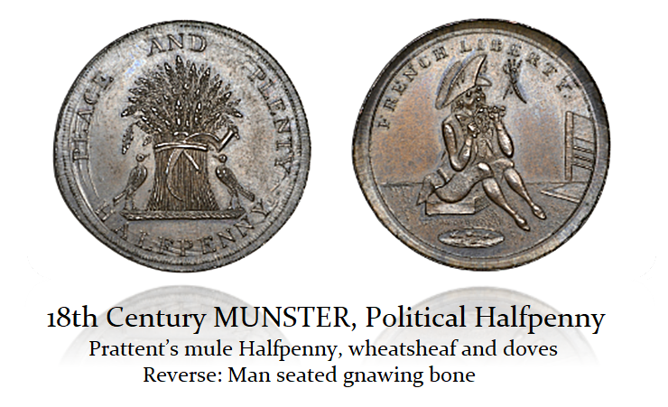
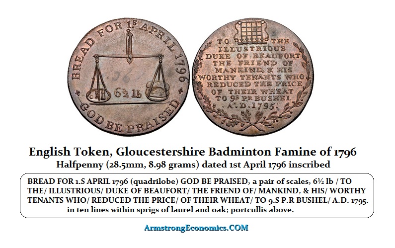
The King of France had listened to the Physiocrats who counseled him to intermittently deregulate the domestic grain trade and introduce a form of free trade. That did not go very well for there was a shortage of grain and this only led to a bidding war – hence the high price of wheat. We even see English political tokens of the era campaigning about the high price of grain and the shortage of food to where a man is gnawing on a bone.

Voltaire once remarked that Parisians required only “the comic opera and white bread.” Indeed, bread has also played a very critical role in French history that is overlooked. The French Revolution that began with the storming of the Bastille on July 14th, 1789 was not just looking for guns, but also grains to make bread.

The price of bread and the shortages played a very significant role during the revolution. We must understand Marie Antoinette’s supposed quote upon hearing that her subjects had no bread: “Let them eat cake!” which was just propaganda at the time. The “cake” was not the cake as we know it today, but the crust was still left in the pan after taking the bread out. This shows the magnitude that the shortage of bread played in the revolution.

In late April and May of 1775, the food shortages and high prices of grain ignited an explosion of such popular anger in the surrounding regions of Paris. There were more than 300 riots and looking for grain over just three weeks (3.14 weeks). The historians dubbed this the Flour War. The people even stormed the place at Versailles before the riots spread into Paris and outward into the countryside.

The food shortage became so acute during the 1780s that it was exacerbated by the influx of immigration to France during that period. It was a period of changing social values where we heard similar cries for equality. Eventually, this became one of the virtues on which the French Republic was founded. Most importantly, the French Constitution of 1791 explicitly stipulated a right to freedom of movement. It was mostly perceived to be a food shortage and the reason was the greedy rich. Thus, a huge rise in population was also contributed in part by immigration whereas it reached around 5-6 million more people in France in 1789 than in 1720.

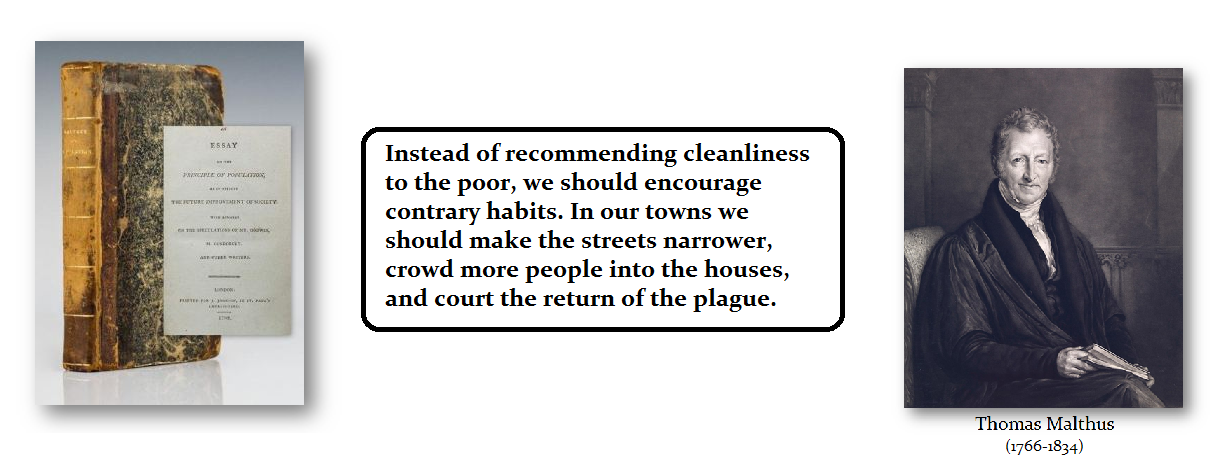
Against this backdrop, we have the publication by Thomas Malthus (1766-1834) An Essay on the Principle of Population was first published anonymously in 1798. He theorized that the population would outgrow the ability to produce food. We can see how his thinking formed because of the Mini Ice Age that bottomed in 1650. All of this was because of climate change which instigated food shortages. Therefore, it was commonly accepted that without a corresponding increase in native grain production, there would be a serious crisis.

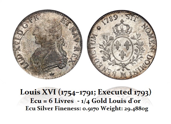
The refusal on the part of most of the French to eat anything but a cereal-based diet was another major issue. Bread likely accounted for 60-80 percent of the budget of a wage-earner’s family at that point in time. Consequently, even a small rise in grain prices could spark political tensions. Because this was such an issue, and probably the major cause of the French Revolution among the majority, Finance Minister Jacques Necker (1732–1804) claimed that, to show solidarity with the people, King Louis XVI was eating the lower-class maslin bread. Maslin bread is from a mix of wheat and rye, rather than the elite manchet, white bread that is achieved by sifting wholemeal flour to remove the wheatgerm and bran.

That solidarity was seen as propaganda and the instigators made up the Marie Antoinette quote: Let them eat cake. . Then there was a plot drawn up at Passy in 1789 that fomented the rebellion against the crown shortly before the people stormed the Bastille. It declared “do everything in our power to ensure that the lack of bread is total, so that the bourgeoisie are forced to take up arms.” 

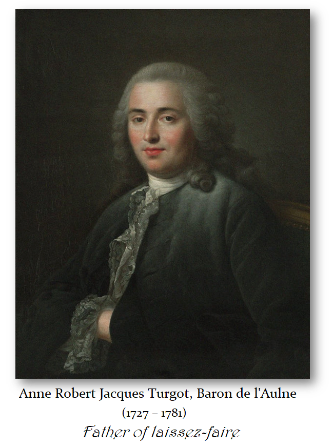
It was also at this time when Anne Robert Jacques Turgot (1727-1781), Baron de l’Aulne, was a French economist and statesman. He was originally considered a physiocrat, but he kept an open mind and became the first economist to have recognized the law of diminishing marginal returns in agriculture. He became the father of economic liberalism which we call today laissez-faire for he put it into action. He saw the overregulation of grain production was behind also contributing to the food shortages. He once said: “Ne vous mêlez pas du pain”—Do not meddle with bread.

The French Revolution overthrew the monarchy and they began beheading anyone who supported the Monarchy and confiscated their wealth as well as the land belonging to the Catholic Church.  Nevertheless, the revolution did not end French anxiety over bread. On August 29th, 1789, only two days after completing the Declaration of the Rights of Man and of the Citizen, the Constituent Assembly completely deregulated domestic grain markets. The move raised fears about speculation, hoarding, and exportation.

Then on October 21st, 1789, a baker, Denis François, was accused of hiding loaves from sale as part of a conspiracy to deprive the people of bread. Despite a hearing which proved him innocent, the crowd dragged François to the Place de Grève, hanged and decapitated him, and made his pregnant wife kiss his bloodied lips. Immediately thereafter, the National Constituent Assembly instituted martial law. At first sight, this act appears as a callous lynching by the mob, yet it led to social sanctions against the general public. The deputies decided to meet popular violence with force.

So, food has often been a MAJOR factor in revolutions. We are entering a cold period. Ukraine has been the breadbasket for Europe. Escalating this war will also lead to accelerating the food shortages post-2024. It is interesting how we learn nothing from history. Wars are instigated by political leaders while revolutions are instigated by the people.

A DIY Guide To Demystifying “Greenhouse Gas” Claims…The Science That Cuts Corners


Reposted from https://notrickszone.com/2023/01/14/a-diy-guide-to-demystifying-greenhouse-gas-claims-the-science-that-cuts-corners/

A DIY Guide To Demystifying “Greenhouse Gas” Claims…The Science That Cuts Corners

By P Gosselin on 14. January 2023

Share this…

By Fred F. Mueller

Do you feel helpless when trying to assess the veracity of “climate doom is looming” claims we are constantly bombarded with?

For ordinary citizens not having acquired at least a Ph.d. degree in atmospheric physics or comparable climate-relevant sciences, it seems nearly impossible to tell right from wrong when it comes to assess such claims. Do so-called greenhouse gases really reflect infrared energy back to earth in such quantities that this affects earth’s temperature?

Don’t give up trying to understand the relevant basics: there are rather simple ways to get an idea about what this is all about. Even without a scientific background, most people have at least a good common sense. And that’s all it takes to get a grasp of how vigorously and chaotically enormous energy fluxes slosh up and down, back and forth between earth’s surface and the skies.

Fig. 1. The setting sun illuminating a fairly thin veil of clouds from below – thus injecting energy into the space between the earths’s surface and cloud cover.

Part 1 – some basics

Let’s first clarify where the heat that allows us to live rather comfortably in our habitats is coming from and where it goes to. Despite the enormous energy content of the molten core of our planet, the bulk of our energy comes from the sun, which sends us energy mainly using three forms of electromagnetic radiation: visible, ultraviolet and infrared light.

At the top of the atmosphere, every square meter oriented towards the sun thus receives a fairly constant power influx of 1361 to 1362 W/m2. Although not being a real constant, this value is often referred to as the solar constant.

The alleged greenhouse effect

The notion of a “greenhouse effect” in our atmosphere has been used and misused incredibly often, resulting in an incredible mess of erroneous perceptions not only among the public, but even in the scientific world. A striking example for an obvious misrepresentation can be seen in the lead-in picture of the Wikipedia chapter on the topic, Fig. 2.

Fig. 2. The lead-in picture of the Wikipedia chapter about the “greenhouse effect” (Author: Efbrazil 2), CC 4.0)

This graphic highlights the extent to which Wikipedia gives the impression of having fallen prey to climate activism. The complex reality of transfers and transformations of energy on our planet involving soils, waters, gases, clouds, aerosols, heat storage, conduction and convection, chemical reactions and phase transformations, as well as a host of additional factors are simply swept under the carpet, attributing all their combined effects solely to the odious “greenhouse gases”.

This Wikipedia chapter is a saddening example for the downfall of an allegedly scientific encyclopedia actually spreading rather crude ideology under the guise of educating the public. The related chapter comprises more than 7,000 words and tries to underscore its claim of being “scientific” by a list of 80 citations including papers about the atmospheric conditions on far-away cosmic bodies such as Titan and Venus. But this cannot excuse the use of such a grossly misleading graphic as the lead-in picture for the abstract. Such tricks commonly used in tabloids or yellow journals. Wikipedia touts itself to be an encyclopedia addressing not only scientists but also laymen and the general public and should therefore care all the more not to disseminate content that may be misunderstood by people lacking a scientific background.

Fig. 3. This more detailed representation of the energy fluxes on earth elaborated by NASA is still misleading with respect to some decisive facts (Picture by NASA 3), public domain) Note: This graphic and the corresponding link have been withdrawn after completion of the article. In a subsequent part, the replacement graphic and its amendments will be treated in detail. Nevertheless, this graphic and its errors have been displayed for a prolonged time, thus warranting a suited discussion.

Although the more detailed Fig. 3 elaborated by NASA gives a better impression of the many different factors influencing energy transfer fluxes between earth’s surface and space, it still misleads in a subtle way that makes it unfit to convey a correct understanding of the vital facts. Let’s look at the main inconsistencies.

Mean values intended to mask natural variations

One of the favourite tricks of climate prophets of doom is to suggest that all major factors influencing our climate are more or less constant, with the sole exception of “greenhouse gases”. They intend to exploit the fact that the CO2-level of the atmosphere is rising while at least for the past some 150 years, meteorologists have also seen a moderate rise of the temperature levels they monitor on their stations. Though both trends are far from being in lockstep, this coincidence of trends has been declared to be the proof for a causality, although no clear mechanism or quantitative deduction could hitherto be established. Despite many striking discrepancies e.g. with respect to the natural cycles of CO2 or the absorption and sequestration of CO2 in our oceans, the perceived rise in temperatures has been almost exclusively attributed to CO2.

Misusing water vapor

Another diversion has been to declare that water vapor is simply reinforcing the leading role of CO2. This might be viewed as a real masterpiece of twisting reality since water vapor has not only a much higher efficiency with respect to absorbing (and re-emitting) infrared radiation (see Fig.4.), but is also exceeds the content of CO2 in the atmosphere by factors between 25 (= median concentration value at sea level) and up to 100!

Fig. 4. Comparing the spectral IR radiance of a surface with 14 °C with the overlapped absorption bands of CO2 (brownish) and water vapor (bluish) shows the highly superior absorption capacity of water vapor for the IR emission of soil or water at 14 °C – (which is the “mean” temperature on earth’s surface). Please mind the different scales of the x axes: linear for the spectral radiance, logarithmic for the absorption. (Graphics: SpectralCalc 4) (above), NASA, Robert Rohde 5) Public domain (below)).

 Notwithstanding these inconsistencies, the climate science community has in its vast majority adopted this approach. This might be attributable to the fact that the quantity of water vapor in the atmosphere is subjected to wild temporal and local variations between nearly zero – e.g. at high altitudes and very low temperatures – and sometimes up to 4% at sea level.

Cutting corners

Additionally, especially when transforming to clouds, water vapor tends to condense or freeze out of the atmosphere in ways that have up to now resisted any realistic attempt to describe them mathematically. Trying to establish realistic three-dimensional models of water vapor distribution over a certain location at a given moment and to calculate the resulting effects on absorption and re-emission of IR radiation thus remain a much more arduous task than using a single value for all and every condition, as can conveniently be done when attributing the whole “greenhouse effect” solely to CO2. And voilà, truckloads of complicated research work may simply be skipped. This approach also greatly reduces the scale of expenditures in data acquisition, manpower, computer time – and in waiting time before reaping academic awards. After all, the beacon for all climate science, the IPCC, is doing it too, e.g. by simply omitting water vapor from its account of “greenhouse gases”, see Fig. 5.

Pic.5. Contribution to observed climate change from 12 different drivers, as taken from the Summary for Policymakers of the sixth IPCC assessment report, adapted from figure SPM.2c (Graphic: Erik Fisk, CC 4.0 6))

The numerous advantages of such a cutting of (scientific) corners might be one of the main driving forces for the deplorable tendency towards the “single number fallacy” explained by Kip Hansen 7) as being “the belief that complex, complicated and even chaotic subjects and their data can be reduced to a significant and truthful single number.”

Unfortunately for us, that’s exactly what the official climate science is doing. Under the headline “One number to track human impact on climate”, NOAA scientists released the first AGGI 8) (aggregated greenhouse gas index) in 2006 as “a way to help policymakers, educators, and the public understand the cumulative impact of greenhouse gases on climate over time”.

The minuscule driving forces of “greenhouse gases”

When trying to assess the real impact of “greenhouse gases” on earths energy balance, the first step should be to assess the driving force they are alleged to exert on the input and output of energy fluxes. Corresponding parameters can be found in a table within the Wikipedia chapter about Greenhouse gases 9). They reveal that in the view of the leading climate scientists, just four gases have a relevant influence on the budget of energy exchange between incoming and outgoing radiation energy since the alleged start of “human- induced climate change” in 1750. These are:

Carbon dioxide with                          + 2.05    W/m2
Methane with                                      + 0.49    W/m2
Nitrous oxide with                             + 0.17    W/m2
Tropospheric ozone                           + 0.4      W/m2
===========
Total GHG contribution             +3.11     W/m2

This figure is extraordinarily small when comparing it with the enormous temporal and local variability of energy fluxes within our planet’s ocean/atmosphere/soil system within short time periods, and amounts to just a low single digit percentage of the daily variations. This will be treated in more detail in the following chapter.

Peculiarly enormous greenhouse effect range 

On a side note, it is interesting to see that the IPCC gives an enormous range for the greenhouse effect (TCR, Transient Climate Response or “climate sensitivity10)) of CO2, which is estimated to range “likely” between 1.5 and 4.5°C. The figure represents the alleged rise of earth’s mean temperature in °C for every doubling of the CO2 level of the atmosphere. Given this extraordinarily broad range of ± 50%, one might be surprised that IPCC, NOAA and Wikipedia authors advance temperature rise values for greenhouse gases calculated with up to three “significant” digits. This too might be attributable to the feeling of certainty about climate relevant figures instilled into the public by the “one number fits it all” mentality prevalent in our current climate science community.

References

  1. https://en.wikipedia.org/wiki/Solar_constant
  2. https://en.wikipedia.org/wiki/Greenhouse_effect
  3. http://science-edu.larc.nasa.gov/energy_budget/pdf/Energy_Budget_Litho_10year.pdf (Note: This link seems to have been deactivated very recently.)
  4. https://www.spectralcalc.com/blackbody_calculator/blackbody.php
  5. File:CO2 H2O absorption atmospheric gases unique pattern energy wavelengths of energy transparent to others.png – Wikimedia Commons
  6. https://commons.wikimedia.org/wiki/File:Physical_Drivers_of_climate_change.svg
  7. https://wattsupwiththat.com/2023/01/03/unknown-uncertain-or-both/
  8. https://research.noaa.gov/article/ArtMID/587/ArticleID/2877/Greenhouse-gas-pollution-trapped-49-more-heat-in-2021-than-in-1990-NOAA-finds
  9. https://en.wikipedia.org/wiki/Greenhouse_gas
  10. https://www.metoffice.gov.uk/research/climate/understanding-climate/climate-sensitivity-explained

Two More Bodies Recovered in Aftermath of Hurricane Ian


Posted originally on the CTh on January 14, 2023 | Sundance

Their names will not make national headlines, and generally everyone has moved on, but to their families and friends Ilonka Knes and James Hurst mattered.  As CTH readers may remember, in the aftermath of Hurricane Ian we shared that many missing people would be found in the months after the storm, and unfortunately many more will likely never be found.

The body of Mrs Ilonka Knes (82) was found in the mangroves and back bay salt marsh near Fort Myers Beach and has been positively identified. The body of her husband Robert was found in the days immediately following Hurricane Ian.

Additionally, the sailboat “Good Girl” was found submerged with human remains believed to be the body of James ‘Denny’ Hurst (73).

Mrs. Knes and Mr Hurst bring the total number of Hurricane Ian victims in Lee County, Florida, to seventy-five.  Mr. Hurst was the final “official” missing person on the local list; however, there are many more yet unaccounted that were not from this immediate area.   The physical devastation is widespread, but the emotional toll on the families and friends of the missing has been beyond imagining.  Tonight, two more families have answers.

(FLORIDA) – During Thursday’s news conference, Lee County Sheriff Carmine Marceno released new information regarding the area’s recovery.

“Most of us have gotten back to a sense of the new normal. For some, still missing their loved ones, every day since the storm has been difficult,” said Marceno.

The sheriff said his agency originally attempted a well-being check at what was left at the home of Ilonka and Robert Knes in the aftermath of the storm.

The body of Robert Knes was found shortly after Ian struck, but there were no signs of his wife during the days and weeks following the disaster.

Marceno said it wasn’t until mid-January that a debris removal crew found remains in a dense patch of mangroves, that later tested positive, through the use of dental records, to be that of Ilonka. (more)

The power and duration of Hurricane Ian killed more people than Hurricane Andrew and the storm that hit Southwest Florida last September is now recorded as the deadliest storm in the past 87 years.

If you live anywhere along the coastline of the United States, inland to about 50 miles, please remember to always take these storms seriously.

After this storm, and having been through four previous direct impacts, including Homestead AFB (Andrew), I would say this….  If there is even a remote chance you would ever encounter this type of a hurricane event, EVACUATE.  Do not try and hunker down if there is a looming possibility of having to rely on a structure to withstand 150+ mph wind for a full day.  Just leave.  With all of my preparations in place, and all of the knowledge I possess in storm survival, I would never attempt it again.

It is more than three months since Hurricane Ian hit Southwest Florida and beyond the chaos and debris that still remains visible almost everywhere, they are still recovering bodies.  Please take hurricane preparations seriously.

Lessons from Ian – Part One

Lessons from Ian – Part Two

Time to talk about capacity factors


It is Time to Talk About “Capacity Factors”

January 12, 2022

Dr. Lars Schernikau, energy economist and commodity trader, Switzerland/Singapore, https://www.linkedin.com/in/larsschernikau/

It is time to talk about “Capacity Factors”​

In electricity generation, capacity factor, utilization, and load factor are not the same.

A lot of confusion exists in the press and certainly in politics, and even amongst “energy experts”, about using the term “capacity factor”. It may be excused, since the distinction made in this article became only relevant with the penetration of variable “renewable” energy, such as wind and solar, in our energy systems.

  • Worldwide average solar natural capacity factor (CF) reaches about ~11-13%. Best locations in California, Australia, South Africa, Sahara may have above 25%, but are rare. (see www.globalsolaratlas.info, setting direct normal solar irradiance)
  • Worldwide average wind natural capacity factors (CF) reach about ~21-24%. Best off-shore locations in Northern Europe may reach above 40%. Most of Asia and Africa have hardly any usable wind and the average CF would be below 15%, except for small areas on parts of the coasts of South Africa and Vietnam. (see www.globalwindatlas.info, setting mean power density)

Natural capacity factors in Europe tend to be higher for wind than for solar. Wind installations in Northern Europe may reach an average of over 30% (higher for more expensive offshore, lower onshore), but less than 15% in India and less than 8% in Indonesia.

Average, and the emphasis is on average, annual solar PV capacity factors reach around ~10-11% in Germany, ~17% in Spain, ~25% in California, and may reach 14-19% in India, but they reach less than 15% in Indonesia’s populated areas. Carbajales-Dale et al. 2014 confirm higher capacity factors for wind than for solar; they estimate global average wind capacity factors to be around 21-24% and solar around 11-13% (see figure above).

The figure further below illustrates a two week period in May 2022 (when I wrote this chapter of our book on capacity factors), where the average wind capacity factor reached only ~5% for ALL German wind installations (on- and offshore).


To avoid confusion, I try to use “natural capacity factor” in my writing wherever possible

  •  The “natural capacity factor (CF)” is the % of the maximum possible output of the “power plant” (coal, gas, nuclear, solar, wind, hydro, etc), achieved under the natural conditions of the site, assuming no operational or technological failures or outages.
  • I define “utilization” is the % of the power plant’s workable capacity used on average over the year, which is only reduced because of technological, operational, economical outages or curtailments… completely independent of the CF
  • The “net load factor” – in my definition – is then the product of natural capacity factor x utilization

Thus, when we speak of the natural capacity factor, we are only referring to the nature-derived capacity factor, not the technological or operationally drivenutilization” (often referred to as uptime, plant load factor, or PLF). In other words, when technology fails, or a power plant is turned off on purpose, this will reduce the utilization but not the natural capacity factor.


As mentioned, the natural capacity factor is due to the site, not the solar PV installation. Thus, even a perfect PV material still needs to deal with natural capacity factors with an annual average of 10-25%, not counting for other losses from conditioning, transmission, balancing, or storing highly intermittent sources of electricity (Schernikau and Smith 2021). 

The press has mentioned several times that coal or gas have capacity factors of 60% or less on average. This is at best misleading, more likely knowingly wrong for political reasons. However, such a number is not the nature-derived capacity factor; it is the utilization which declines with higher penetration of wind and solar, and contributes to electricity system cost increases.

Utilization never should and cannot be compared to natural capacity factors, they are very distinct. Conventional power plants have near 100% natural capacity factors, but their operational and technological utilization often falls significantly below 90%, also but not only because of the priority given to wind and solar in the system. Because of their high CF, the net-load factor is only slightly lower than utilization for a convention power plant.

Because utilization of wind and solar is often near 100%, their net-load factor is often only slightly lower than their natural capacity factor.

Figure: Germany’s wind generation 25 April to 10 May 2022 during a 2-week wind lull
Source: Agora 2022, Figure 10 in Book “The Unpopular Truth… about Electricity and the Future of Energy”, http://www.unpopular-truth.com


Needless to say, the natural capacity factor of wind and solar (even for hydro, because of natural river flows) cannot be predicted or guaranteed for any given time frame. The natural capacity factor can be estimated on an annual basis but still varies widely even annually (see Europe in 2021) and is very erratic, sometimes for days and weeks reaching near 0% for wind and solar, even in top locations.

Thus, natural capacity factors worldwide are a direct result of the location of the wind or solar installation; they do not in any way depend on and cannot be influenced by the technology employed.

The last point is important… no technological advances can change the natural availability of wind, solar, or river flows and therefore influence the natural capacity factor for a given installation. Technology CAN and WILL improve how much usable electricity you get out of the natural input product (wind, solar, river flow, gas, coal, uranium, etc)… this is called conversion efficiency and their limits are discussed further below.

Since the easy locations have already been “used up”, one can expect average natural capacity factors to decline over time… contrary to what Net-Zero plans assume (see International Energy Agency (IEA), McKinsey & Company, or International Renewable Energy Agency (IRENA)).

  1. For a photovoltaic (PV) park, the natural capacity factor CF depends entirely on the intensity and duration of the sunlight, which is affected by seasonality and cloudiness, day and night, and the ability to maintain the PV panel surface’s transparency, e.g., dust in the Sahara or snow in winters.
  2. Wind farms’ natural capacity factors depend on the site’s wind speed distribution and the saturation speed of the wind turbine. The CF of a wind turbine is determined by the number of hours per year in which the wind farm operates at or above the saturation wind speed (Smith and Schernikau 2022). If the design wind saturation speed is set low, e.g., 4-5 m/s, the wind farm produces little energy, even for high capacity factors. Typically, wind saturation speeds are 12-15 m/s.

It now becomes obvious why the installed capacity needs to be much larger for wind and solar than for dispatchable power such as nuclear, coal, gas, or hydro. This significant relative increase in energy generation capacity to produce the same available, but unpredictable, energy output is coupled with a significantly higher raw material input and energy input factor for variable “renewable” energy which must be offset from any fuel savings.

#Germany is a good example: Total installed power capacity more than doubled in the past 20 years, essentially all consisting of wind and solar (see figure below)

  • Wind and solar installed capacity is now above 125GW, more than 150% higher than peak power demand in Germany of around 80GW
  • Germany’ conventional installed power capacity consisting of coal, gas, and nuclear still barely matches peak power demand
  • With all this capacity addition in Germany, wind and solar made up less than 30% of total electricity generation in 2021 and about 5% of total energy consumption

Figure: German installed power capacity, electricity production, and primary energy


Source: Schernikau Research and Analysis based on Fraunhofer 2022, AGE 2021, Agora 2022
Figure 7 in Book “The Unpopular Truth…about Electricity and the Future of Energy”, http://www.unpopular-truth.com

The low natural capacity factor of wind and solar installations – without any doubt – is one of the key reasons for their low net-energy efficiency (https://dx.doi.org/10.2139/ssrn.4000800).


On Conversion Efficiency

Below figure summarizes energy conversion efficiencies for wind and solar and the laws they follow. Conversion efficiency measures the ratio between the useful output of an energy conversion machine and the input, in energy terms, thus after accounting for capacity factor.

Figure: Lhttps://i0.wp.com/wattsupwiththat.com/wp-content/uploads/2022/12/image-202.png?w=974&ssl=1aws of physics limit technological improvements for wind and solar
Source: Schernikau and Smith Research and Analysis, Figure 11 in Book “The Unpopular Truth… about Electricity and the Future of Energy”, http://www.unpopular-truth.com

For more Details please see our book “The Unpopular Truth… about Electricity and the future of Energy” (on Amazon)… or www.unpopular-truth.com

This article can also be accessed at

https://www.linkedin.com/pulse/time-talk-capacity-factors-lars-schernikau

Ice Age – the Come Rapidly


Armstrong Economics Blog/Climate Re-Posted Dec 29, 2022 by Martin Armstrong

Spread the love

COMMENT: Marty you may remember this.

When this hit upper midwest I was in middle school in San Diego. I was in the library every morning before school following this, Voyager and Viking.

I watched another rendition of this video on youtube and it cut out the portion where the chief scientist at Lamont-Doherty (Columbia) stated ice-age conditions can return inside of 10-20 years time at any time (or something like that).

Regards

RD, San Marcos Ca

REPLY: With Ice Ages, we find a similar pattern of cyclical pattern formations as we do in markets. About 2.6 million years ago, that is when the Earth entered the Pleistocene period. This was marked by an interesting cyclical pattern whereby there were these deep ice ages that came at regular 43,000-year intervals. Then about 1 million years ago, the Earth entered what is known as the Mid-Pleistocene transition period. It was here where these ice age cycles suddenly expanded from 43,000-year intervals to nearly 100,000-year cycles. The last one was about 11,000 years ago. This is not referring to the Mini-Ice Age of the 1600s.

What we do know is that there were tiny changes in Earth’s orbit. These events are known as Milankovitch cycles. They are believed to have driven the planet in and out of these ice ages. However, it is also now assumed that these Milankovitch cycles have not correlated to the sudden jump in nearly doubling the Ice Age cycle length.

Preliminary data from Antarctic Ice Core saw a transition from glacial to interglacial conditions about 430,000 years ago which is known as (Termination V). This transition into the present interglacial period needs to be looked at from intensity using our Energy Models. Scientists look at the magnitude of change in temperatures and greenhouse gases. What seems to be overlooked is the cycle of these warming periods. The interglacial stage following Termination V was quite long running the course of about 28,000 years compared to the 12,000 years period so far in the present interglacial period.

What this is warning is that an Ice Age is not entirely out of the question post-2032. I am awaiting access to the data from the 2.7 million-year core and then run it through Socrates to see if we are indeed going to see a 12,000-year interval or a doubling effect. What does appear to be likely, which explains the frozen animals in Siberia, is that we can see an Ice Age hit within less than 10 years.