The FED is now TRAPPED Between the ROCK and the HARD PLACE


Yellen Is Trapped in the Worst Nightmare Ever

yellen-Janet

Yellen has inherited a complete nightmare. Thursday’s decision to delay yet again the long-awaited liftoff from zero interest rates is illustrating that the world economy is totally screwed. There is a lot of speculation about why the Fed seems so reluctant to “normalize monetary policy”. There are of course the typical domestic issues that there is low inflation, weak wage gains in the face of strong job growth, a hike will increase the Federal deficit and then there is the argument that corporations that now have $12.5 trillion in debt. All that is nice, but with corporate debt, our clients are locking in long-term at these levels, not funding anything short-term. Those clients who have listened are preparing for what is to come unlike government which has been forced to shorten the average duration of their debts blind to what happens when rates rise, which will be set in motion by the markets – not Yellen.

Fed is really caught between a rock and a very dark place. Yes, they have the IMF and the world pleading with them not to raise rates for it will hurt other debtors who borrowed excessively using dollars to save money. The Fed is also caught between domestic policy objectives that dictate they MUST raise rates of they will bankrupt countless pension funds and international where emerging markets will go into default because commodities have collapsed and they have no way of paying off this debt that has risen to about 50% of the US national debt.
By avoiding the normalization of interest rates (hikes), the Fed has encouraged government to spend far more than they realize because money is cheap. This will eventually light the fire under the economy helping to fuel the Sovereign Debt Crisis. There appears to be no hope for the Fed and they will be forced to raise rates only when they see asset inflation in equities. Then they will have no choice. This is the worst possible mess and the longer they have waited to normalize interest rates, the worst the total crisis is becoming for they will have zero control over the economy and once that is seen, holy Hell will break lose.

There is no end to the ways the Government can Confiscate your Wealth


Sovereign Debts: How Defaults May Unfold

Germany_bonds

In the Middle East, the banks are trying to convince the Gulf States to begin issuing debt even if there is no need to borrow, simply so they have a market to trade. Governments should never listen to bankers for this always becomes a conflict of interest with respect to national debts. The sooner government wakes up to the Sovereign Debt Crisis, the soon their particular country will be saved.

When you say we are entering a “Sovereign Debt Crisis”, people automatically assume that debt will just default. Governments NEVER like to admit a mistake, so an outright default may be limited to the emerging markets the further you move away from the core economies. What may also take place is the mandatory conversion of debt extending the maturity. You may buy 90-day paper and suddenly wake up to find that the government has converted 90-day paper into 10-year bonds. Always remember, they have the tanks and guns — never forget whom you are dealing with.

In Italy, the period 1919–1922 was one of very little progress on debt and deficit reduction. Despite a levy on wealth that was introduced to tax the rich, as always, the tax faced tremendous opposition as well as implementation difficulties. Consequently, Italian fiscal deficits remained high, and inflation increased along with the money supply rather significantly. The Italian government engaged in a mandatory debt conversion, known as “conversione forzosa” during 1926, which they would again impose during 1934. They forced debt holders to extend their debt by lengthening the maturity. This seriously impacted the full faith and trust in the Italian government. During the post-1926 years and then again after 1934, the mandatory conversione forzosa effectively was seen as a partial default by the government, which made it extremely difficult and costly to borrow on a short-term basis thereafter.

You must be careful in the post-2015.75 era. Owning even short-term government paper can result in a conversione forzosa, which is the usurpation of capital by sheer force. This is one form of default that people need to realize has also been a means of default. The City of Detroit suspended all debt payments between 1937 and 1963. Britain entered a moratorium in 1931 on its debt, resuming years later.

Consequently, defaults, suspensions, moratorium, and conversione forzosa are different types of defaults whereby you lose access to your capital. There are many different flavors of a Sovereign Debt Crisis.

Are NASA-GISS Published Global Temperatures Valid?


NASA publishes values representing the global surface temperature of the planet supposedly based on actual measurements processed in a complex algorithm they call homogenization. The resulting values are published each month in a table called the Land Ocean Temperature Index (LOTI) which runs from January 1880 to the current month, May in this case. The process they use is explained on their web site for those that are interested. However the values shown in their work seem to show very large temperature swings on a month to month basis and that did not seem reasonable to me, given this was Global temperatures. This prompted me to do a review of the process in June 2015 and that led to a previous draft paper which was modified to create this finished work.

A small sample from NASA’s table is provided below running from January 2001 to May 2015. A good example of this large swing in values can be found in the value shown in February 2014 of 44 compared to March 2014 of 71 (both shown in red) a difference of 27 anomalies, a NASA measure of temperatures in hundredths of a degree Celsius, represents a lot of energy on a global scale.

000 CHART OOO

What we are going to do now is reverse engineer the NASA Temperature values in the full LOTI table and then calculate the energy flows required to make those changes. If the “required” energy flows are not reasonable, then the NASA temperatures are not reasonable. They must be in synchronization with each other as energy can neither be created nor destroyed. The first step was to place all 1925 LOTI values in a spreadsheet and then turn the NASA anomalies (a deviation from a base of 14.0 degrees Celsius) back into temperatures by dividing by 100 then adding that value back to the base 14.0 degrees Celsius and lastly adding that result to 273.15 to convert to degrees Kelvin. Kelvin must be used to calculate total heat when working on these kinds of projects.

Next we needed to calculate the total heat value of the NASA temperatures and their changes and so from Wikipedia we find that the Earth’s dry atmosphere is 5.1352E+18 kg and the water in the atmosphere is 1.27E+16 kg for a total of 5.1479E+18 kg. From these values we can calculate that water is on average .247% of the atmosphere. We also find that on Wikipedia the specific heat of the Earth’s atmosphere is 1006 Joules per degree Kelvin (J/kg/K) without water and so we need to add 4.6 J/kg/K for water and 9.8 J/kg/K for latent heat to the 1006 J/kg/K giving us a total of 1020.4 J/kg/K for the earth’s atmosphere with .0247% water at standard air.

There is one last step since the NASA values are “surface” temperatures, we need an adjustment for altitude cooling if we are looking for the total energy in the atmosphere. To accomplish this we’ll subtract 28.5 degrees Celsius making the answer the theoretical temperature at 5 km above sea level which is about where 50% of the atmosphere is above 5 km and 50% below; so this makes for a reasonable estimate for calculating total energy. Using this logic we subtract the 28.5 degrees Celsius from the NASA LOTI values that we converted to degree Celsius, which are surface values which then gives a ballpark value to calculate the total heat in the atmosphere.

With the monthly NASA temperatures in a spreadsheet it was only a few hours work to set up the equations and plot a few charts. We calculated the heat value of each month’s anomaly for example for January 1880 the value was 1.3572E+24 Joules and for June 2015 the value was 1.36266E+24 Joules. Those values are a result of energy coming in from the sun minus what leaves the planet as infrared energy assuming no large change in the temperature of the land or oceans. To my knowledge these kinds of temperature changes (energy flows) have not been observed on the surface of the planet.

This review shows that the magnitude of the “required” energy flows is not reasonable indicating to me that the NASA temperatures is not reasonable as can be seen in Chart 1 on the next page. This shows two plots, the monthly change in the NASA anomalies in blue (required energy out) and the sun’s input in red (energy in). The sun’s input is adjusted for the orbital distance to the sun and the number of days in the month which is required to match the time periods shown in the NASA LOTI table. Since the sun is the energy input, the NASA temperatures minus the input must equal the input with the opposite sign, or negative. In other words, the sum of the two must be zero.

, David Pristash

It’s clear when looking at Chart 1 that there have to be extremely large monthly energy flows involved here if the NASA numbers are actually valid. To put this in perspective three, lines were added to Chart 1, as shown in Chart 2. These lines are for the incoming solar radiation using 1414.44 Wm2 for solar radiation at aphelion (January) and 1322.97 Wm2 for solar radiation at perihelion (July) in the earth’s orbit using the following albedo percentages; 20.0% dark red plot, 30.0% (Actual) red plot and 40.0% a yellow plot. The red plot is also shown on Chart 1. We also changed the time frame from 1880 to the present to 2000 to the present so that more detail could be seen when making Chart 2.

The choppy lines in the dark red, red and yellow Sun radiation plots are a result of using monthly values and the months don’t always have the name number of days. The purpose of showing these three radiation plots from the sun is to show that large changes in the planets albedo cannot account for the large energy swings and so the large changes in the NASA data such as shown here just don’t happen. That means that even these large albedo changes cannot account for the large required movements in energy indicated by NASA’s numbers shown in their table LOTI, the actual smaller albedo changes we experience surely can’t.

00 NASA REVIEW-02

The blue plot for the NASA temperatures is actually the “required” energy out flow to balance the suns energy inflow. Given the process that NASA uses to determine global temperatures it would be expect that there would be some variations, but surely not of the magnitude shown in this chart.

NOAA and NASA have spend a lot of time and resources developing complex systems with the intent to show how “current’ temperatures were being driven up by the level of greenhouse gasses in the atmosphere caused by the burning of fossil fuels. This was called anthropogenic climate change meaning climate change caused by man. These apparent upward global temperature changes in the 1980’s and 1990’s were assumed by politicians to be dangerous and the scientific community given the task of showing the dangers to the planet of increasing temperatures. Although there was some real scientific validity to the man made climate change movement a true cause and effect review of the concept was never made and money poured in to “prove’ the concept.

Had a true review of the apparent problem been done first it would have been obvious that there were other factors involved besides greenhouse gases the most obvious was the well documented thousand year cycle of warm and cold periods going back several thousand years. The most recent of these cycles ended around 1650 during the coldest part of what is called the Little Ice Age. Assuming the thousand year cycle is valid that means that the global temperature would be ascending for five hundred years peaking around 2150. Based on this principle of multiple reasons for the apparent climate change, a climate model was then developed that fit the historic patterns that includes the increases in greenhouse gases. This model is called a pattern model and designated the PCM and shown next.

000 2015-06 b

The next Chart 1a was developed exactly the same way as the NASA Chart 1 was except we used the temperatures generated by the PCM model as shown in the previous PCM chart instead of those developed by NASA in their computer system. We can clearly see in this Chart 1a that this PCM model generates a plot that very closely matches the suns input but is negative which it must be to keep the planet in thermal balance.

00 NASA REVIEW-05

The next Chart 2a is based on the same principle as that shown for the NASA data in Chart 2 looking at 2000 to the present for more detail and we can see that the sun’s is exactly balanced by the energy leaving the planet as it must be when we use the PCM model to generate the temperatures. The model was developed in 2007 and this review used the values calculated by the PCM model.

00 NASA REVIEW-04

Further from a total energy, heat, perspective the current increase in global temperatures of just over plus 1 degree Celsius from 1880 is less than 4 tenths of a percent change in the planets heat content. Even 2 degrees Celsius as predicted by the PCM model would be less than 6 tens of a percent change in the planets heat content so making claims of utter disaster for such small amounts of a heat increase is really stretching the point especially since the planet has reached temperatures beyond where we are now many times in the distant past; we are still just barely out of the last ice age after all.

The point to this analysis is to show that whatever the method used to analyze global temperatures, the in’s and out’s must balance. Clearly the NASA-GISS table LOTI data is not valid for the monthly temperature swings exceed what would be possible in the real world. Maybe if NASA would concentrate on developing real systems and models instead of doing the bidding of politicians their work might actually be valid.

This paper contains original research on the energy balance of the climate (weather) of the planet. A more sophisticated analysis could possibly be done showing what the effect of the1 to 2 degree Celsius increase in global temperatures that has accrued since the end of the little ice age in ~1650 would look like; maybe a 3D chart would work giving another dimension to work with. The energy balance would still be there but the in’s and out’s would have a pattern similar to what is shown in the chart of the PCM model and trending upward indicated that there is an increase in temperature

Analysis of Global Temperature Trends, August, 2015 What’s really going on with the Climate?


The analysis and plots shown here are based on the following: first NASA-GISS temperature anomalies (converted to degrees Celsius so non-scientists will understand the plots) as shown in their table LOTI, second James E. Hansen’s Scenario B data, which is the very core of the IPCC Global Climate models (GCM’s) and which was based on a CO2 sensitivity value of 3.0O Celsius, lastly, a plot based on an alternative climate model designated ‘PCM’ and based on a sensitively value of 0.65O Celsius.

An explanation of the alternative model designated, PCM, is in order since many have interpreted this PCM model as a statistical least squares projection of some kind. Nothing could be further from the truth. A decade ago when I started this work the first thing I did was look at geological temperature changes since it is well known that the climate is not a constant; I learned that in my undergrad geology and climatology courses in 1964.

The following observations give a starting point to any serious study. First, there is a clear movement in global temperatures with a 1,000 some year cycle going back at least 3,000 to 4,000 years; probably because of the apsidal precession of about 21,000 years for a complete cycle. However about every 10,000 years the seasons are reversed making the winter colder and the summer warmer in the northern hemisphere. 10,000 years from now the seasons will be reversed. Secondly, there are also 60 to 70 year cycles in the Pacific and the Atlantic oceans that are well documented. Lastly we also know that there are greenhouse gases such as carbon dioxide. The National Academy of Sciences (NAS) estimated that carbon dioxide had a doubling rate of 3.0O Celsius plus or minus 1.5O Celsius in 1979.

The core problem with the current climate change theory is that the IPCC still uses the NAS 3.0O Celsius as the sensitivity value of carbon dioxide and a number in that range is required to make the IPCC GCM’s work. The problem with using this value is it leaves no room for other factors and hence the need of the infamous hockey stick plots of the IPCC from Mann, Bradley & Hughes in 1999. The PCM model is based on a much lower value for carbon dioxide consistent with current research. This places the value between 0.65O and 1.5O Celsius per doubling of carbon dioxide. If the long and short movement in temperatures and a lower value for carbon dioxide are properly analyzed and combined a plot that matched historical and current (non manipulated) NASA temperature estimates very well can be constructed. This is not curve fitting.

The PCM model is such a construct and it is not based on statistical analyses of raw data. It is based on creating curves that match observations (which is real science) and those observations appear to be related to the movement of water in the world’s oceans. The movements of ocean currents are well documented in the literature. All that was done here was properly combine the separate variables into one curve which had not been previously done, to my knowledge. Since this combined curve is an excellent predictor of global temperatures unlike the IPCC GCM’s, it appears to reflect reality a bit better than the convoluted IPCC GCM’s, which after the past 19 years of no statistical warming have been shown to be in error.

Now, to smooth out highly erratic monthly variations a 12 month running average is used in all the plots. This information will be shown in four tables and updated each month as the new data comes in about the middle of the month. Since no model or simulation that cannot reasonably predict that which it was design to do is worth anything the information presented here definitively proves that NASA, NOAA and the IPCC just don’t have a clue.

000 2015-06 a

The first plot, UL is a plot of the NASA temperature anomaly converted to degrees Celsius and shown in red with a black trend line added. There has been a very clear reversal in the upward movement of global temperatures since about 2001 and neither the UN IPCC nor anyone else has an explanation for this 13 years later. Since CO2 has continued to increase at what could be argued an increasing rate, this raises serious doubts about the logic programmed into all the IPCC global climate models.

The next plot UR, also in red, shows the IPCC estimates of what the Global temperature should be, based on Hansen’s Scenario B, with the NASA actual temperatures’ subtracted from them. Therefore this plot represents a deviation from what the Climate “believers” KNOW what the temperature should be; with a positive value indicating the IPCC values are higher than actual and a negative value indicating the IPCC values are lower than actual, as measured by NASA. A black trend line is added and we can clearly see that the deviation from expected is increasing at an increasing rate. This makes sense since the IPCC models project increased temperatures based primarily on the increasing level of CO2 in the earth’s atmosphere. Unfortunately, for them, the actual temperatures from NASA are trending down (even as they try to hide the down ward movement with data manipulation) since other factors are in play, therefore each year the gap between them widens. Since we have 13 years of observations’ showing this pattern it becomes hard to justify a continuing belief in the IPCC climate models, there is obviously something very wrong here.

The next plot LL shown in blue is based on the equations in the PCM climate model described in previous papers and posts here and since it is generated by “equations” a trend line is not needed. As can be seen the PCM, LL, and the NASA, UL, trend plots are very similar the reason being that in the PCM model, there is a 68.2 year cycle that moves the trend line up and then down a total of 0.30O Celsius (currently negative .0070O Celsius per year); and we are now in the downward portion of that trend which will continue until around 2035. This short cycle is clearly observed in the raw NASA data in the LOTI table going back to 1868. Then there is a long trend, 1052.6 years with an up and down of 1.36O Celsius (currently plus .0029O Celsius per year) also observed in the NASA data. Lastly, there is CO2 adding about .005O Celsius per year so they basically wash out, which matches the current holding pattern we are experiencing. However within a few years the increasing downward trend of the short cycle will overpower the other two and we will see drop of about .002O Celsius per year and that will be increasing until till around 2025 or so. After about 2035 the short cycle will have bottomed and turn up and all three will be on the upswing again. These are all round numbers shown here as representative values.

The last plot LR in blue uses the same logic as used in the UR plot, here we use the PCM estimates of what the Global temperature should be with the NASA actual temperatures’ subtracted from them. A positive value indicates the PCM values are higher than actual and a negative value indicates the PCM values are lower than expected. A black trend line was added and it clearly shows that the PCM model is tracking the NASA actual values very closely. In, fact since 1970 the PCM model has rarely been off by more than +/- 0.1 degrees Celsius and has an average trend of almost zero error, while the IPCC models are erratic and are now approaching an error rate of +0.5O above expected.

Note: Since I first started posting this monthly analysis a year and a half ago NOAA and NASA were directed make the global temperatures fit the political narrative that the planet was over heating and something drastic need to be done right now. The problem was as shown in this analysis the “real” world temperatures were not at the level that the IPCC GCM’s said they should be. Major adjustments to the data have been made that give the illusion that temperatures are going up even though they are not. However, as this analysis shows even with the manipulation that has destroyed all credibility from NOAA and NASA they cannot get the global temperatures even close to what their false theory claims they should be.

In summary, the IPCC models were designed before a true picture of the world’s climate was understood. During the 1980’s and 1990’s CO2 levels were going up and the world temperature was also going up so there appeared to be correlation and causation. The mistake that was made was looking at only a ~20 year period when the real variations in climate move in much longer cycles. Those other cycles can be observed in the NASA data but they were ignored for some reason. By ignoring those trends and focusing only on CO2 the models will be unable to correctly plot global temperatures until they are fixed.

Lastly, the next chart shows what a plot of the PCM model would look like from the year 1000 to the year 2300. The plot matches reasonably well with history and fits the current NASA-GISS table LOTI date very closely, despite homogenization. I understand that this model is not based on physics but it is also not curve fitting. It’s based on observed reoccurring patterns in the climate. These patterns can be modeled and when they are, you get a plot that works better than any of the IPCC’s GCM’s. If the conditions that create these patterns do not change and CO2 continues to increase to 800 ppm or even 1000 ppm than this model will work into the foreseeable future. 150 years from now global temperatures will peak at around 15.5 to 15.7 degrees C and then will be on the downside of the long cycle for the next 500 years. The overall effect of CO2 reaching levels of 1000 ppm or even higher will be between 1.0 and 1.5 degrees C which is about the same as that of the long cycle.

Carbon Dioxide is not capable of doing what Hansen and Gore claim!

000 2015-06 b

The purpose of this post is to make people aware of the errors inherent in the IPCC models so that they can be corrected.

The Obama administration’s “need” for a binding UN climate treaty with mandated CO2 reductions in Europe and America means there will be such a resolution presented at the COP12 conference in Paris in December. To support this NASA will be forced to show ever increasing global temperatures for the rest of 2015 that will make less and less sense based on observations and satellite data which will all be dismissed or ignored.

Sir Karl Raimund Popper (28 July 1902 – 17 September 1994) was an Austrian and British philosopher and a professor at the London School of Economics. He is considered one of the most influential philosophers for science of the 20th century, and he also wrote extensively on social and political philosophy. The following quotes of his apply to this subject.

If we are uncritical we shall always find what we want: we shall look for, and find, confirmations, and we shall look away from, and not see, whatever might be dangerous to our pet theories.

Whenever a theory appears to you as the only possible one, take this as a sign that you have neither understood the theory nor the problem which it was intended to solve.

… (S)cience is one of the very few human activities — perhaps the only one — in which errors are systematically criticized and fairly often, in time, corrected.

A Serious Proposal for a different method of funding government operations suitable for a technology based economy


money wave

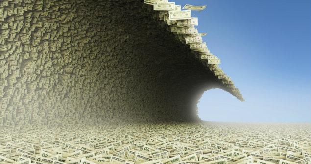
The Federal government never has enough money and over the past decade they have created enough money, Dollars, that there is a title wave of them about to hit us; we need a different system that the politicians can’t subvert. This short post is a way to achieve that.

The following figures are taken directly from the following government reports: Bureau of Economic Analysis (BEA) monthly report of the GDP of the United States; Monthly Treasury Statement; the Bureau of Labor Statistics (BLS) monthly employment situation; The Monthly Statement of the Public Debt of the United States and the Department of Defense (DOD) Active Duty Military Strength Report. The Monthly Treasury Statement data is reformatted to calendar year format the government fiscal year format which runs from October to September so we can compare apples to apples.

First the Facts for 2014:

#1 The federal government currently spends almost $4.0 trillion a year ($3.885 trillion) of which some is derived from taxes & fees ($3.096 Trillion) and some is borrowed ($789.5 Billion). More on this subject later since the official GDP figures are different; so we use $3.2 Trillion here instead of the actual $3.9 Trillion, to be consistent with BEA numbers (explained later).

#2 There are some 151,012,000 people working for a living including ALL categories (the BLS does not count farm, self-employed and the military). This figure is the average for the calendar year 2014.

#3 If we assume there are 2,000 hours worked per year per person that equates to 302 billion hours worked per year. This is the only assumption used here and since many workers are part time this maybe an overstated number. Whether it is or not doesn’t matter to the discussion of the concept. It would only matter if implemented.

# 4 Therefore, if we divide the $3.2 Trillion spent by the Federal government by the 302 billion hours worked by all the citizens, that gives a ratio of $10.56 of federal spending per hour worked.

Now here is the concept:

The idea is based on an economic principle that my advanced econ professor taught me my senior year at Ohio University which is, basically just a form of a thought experiment. The principle is that if we make a change and the result of the change shows a result that is the same as before the change, then there was no real change in the output only a change in how we got there. The assumption then is that it makes no difference which method is used.

What follows is for federal spending only, state and local could also be added to this but that is too complex for this brief overview. This does include ALL revenue going to the federal government no matter the reason or program including social security.

#1 We eliminate ALL personal federal taxes and fees and ALL business taxes and fees as well which then reduces the governments’ income to zero (all borrowing is also eliminated).

#2 Simultaneously we reduce individual pay rates by the exact amount of the taxes they pay. For example if you were making $25.00 per hour but only taking home $20.00 per hour the change we make would be that you would now be making $20.00 per hour but paying no taxes so your take home would be the same as before $20.00 per hour (no change).

#3 Businesses would be required to reduce prices such that their income would be unchanged in a similar manner. So the net economic effect on the economy from this change (initially) would be zero since private and corporate spending would be exactly the same (no change).

#4 To compensate for this loss of revenue the federal government would be allowed to create fiat money (no real change from what they do now) at the rate of $10.56 per hour worked by the citizens.  And since there would still be 302 billion hours worked by the citizens (no change) they could spend $3.2 trillion dollars (no change).

$5 The result is that there is still the exact same amount of money in the economy in both the current system and the new system. All we did is change the method of how it got from the worker to the government.

You can see we have made major changes but nothing has really changed, we just changed the method of how we got from there to here. So therefore we are in accordance with the economic principle we started this section with being true.

I think you can see the benefits to this kind of system and, of course the devil is always in the details; however I believe I have considered most of them and they are not major obstacles. I do agree that this would take a lot of re-education to the public but I think it could be sold especially after 2017.
The major benefits are:

#1 The federal government can only spend more money when there are more people working more hours. That is an incentive to promote growth not dependency.

#2 No one has to worry about paying federal taxes so all purchasing and investment decisions are based on economics not tax avoidance. This makes for a much more efficient economy.

#3 The federal budget is always in balance. No need to borrow money and this also forces international trade to be in balance since the government doesn’t need to borrow from foreigners.

#4 Lower prices for products produced here would make the US more competitive and since the take home income is the same internal growth would be immediate.

#5 We end up with a labor based currency which is a improvement over what we have which is debt based. It also takes gold out of the equation except possibly for international trade since the current system we have of pegged rates does not work. However, that is a different subject for other papers.

#6 There are no downsides other than some federal agencies would no longer be required, such as the IRS and the FED. So actually the federal government would need less money.

The Equations:

The equations shown after this discussion are used in national income accounting to calculate Gross National Product (GDP). To show how this works we present an example using the real numbers for 2014. Again this is a simple macro model and the details are much more complicated then what is shown here. However, that doesn’t matter since the principle is valid and all the details can be worked out.

Note the BEA does not count borrowed money and transfer payments are not shown as growth. The BEA’s G also includes state and local spending much of which is transfer payments from the federal government. This means that the BEA figures for “government” used to calculate the GDP are not the same as shown by the United States Treasury for federal spending and borrowing. We will use the BEA figure of $3.2 Trillion instead of the actual $3.9 trillion pulled from the economy by the federal government for 2014 in this exercise.

GDP = Y = C + I + G + (X – M)

GDP = Y = $17.7 = $12.1 + $2.9 +$3.2 + ($2.4 – $2.9)

Where C (consumption net of taxes CN) can be defined as gross income (Cg) less federal taxes (TF) or CN= CG – TF

Where I (investment net of Federal borrowing or IN) can be defined as gross investment (IG) less federal borrowing (BF) or IN = IG – BF

Where G (government) can then be defined as government taxes (TF) + government borrowing (BF)

X is exports

M is Imports

Y = CN + IN+ G + (X – M) or

Y = CN + IN + TF+ BF + (X – M)


After the proposed change

CG = CN

IG = IN

G = Hours worked (HW) * $10.56

GDP = Y = CN + IN + G + (X – M)

GDP = Y = CN + IN + 10.56 * Hw + (X – M)

GDP = Y = CN + IN + (10.56 * .302) + (X – M)

GDP = $17.7 = $12.1 + $2.9 +$3.2 + ($2.4 – $2.9)

Obviously nothing has changed since in either the old method or the new method The GDP = $17.7 trillion. Properly packaged, presented and sold by someone would solve many of our problems and doesn’t hurt either conservative or liberal principles.

Notes and Comments:

Federal Spending is very different from what is generally shown or known, for example: The Monthly Treasury Report for 2014 (adjusted to a calendar year) Shows the Federal Government spent $3.585 Trillion dollars derived from $3.096 Trillion from taxes and fees and $667 billion from borrowing. However the National Debt during the same period went up by $789 Billion so there was additional cash needed for changes in payables and obligations and capital projects of $122 Billion. Therefore the federal government actually spent/used $3.885 Trillion in 2014 or 21.95% of the GDP.

Also as previously mentioned transfer payments to the states and cities i.e. block grants do not show as being Federal spending in GDP analysis. That is unfortunate since the federal government has strings attached which give them control of the money and that will get much worse after 2016 when the full force of the Affordable Health Care Act goes into effect.

The purpose of the quick review of my idea is to show that economically and monetarily this system works. It works because economics is about people and what motivates them. In one sense Karl Marx was right labor is the ultimate source of value, he was wrong in how to use that principle and that wrongness has lead to much suffering in the world as we tried to absorb his idealist thoughts (socialism) into the real world.

This proposed system is a method of merging both Adam Smith and Karl Marx while rejecting John Maynard Keynes completely.

Hillary’s Deceit and lies go all the way back to 1974


In 1974 President Nixon resigned from his position as the President of the Unites States, in part from the threat from the House of Representatives that they would impeach him. Whether he would have been or not his demise was, in part, a result of the then young 27 tear old staffer Hillary Rodham who married William Clinton the next year.

The following link will give you are the gory details and that are not faltering to Hilliary who was a consummate lair even back then.

By DAN CALABRESE – Bet you didn’t know this

Wouldn’t it be poetic Justis if what Hilliary did in 1974 to bring down Nixon detailed her presidential campaign for erasing a hard drive to hide her crimes in 2015 some 41 years after accusing Nixon of hiding his crimes by easing tapes started her career that lead her to this spot.


Analysis of Global Temperature Trends, July 2015 What’s really going on with the Climate?


The analysis and plots shown here are based on the following: first NASA-GISS temperature anomalies (converted to degrees Celsius so non-scientists will understand the plots) as shown in their table LOTI, second James E. Hansen’s Scenario B data, which is the very core of the IPCC Global Climate models (GCM’s) and which was based on a CO2 sensitivity value of 3.0O Celsius, lastly, a plot based on an alternative climate model designated ‘PCM’ and based on a sensitively value of .65O Celsius.
An explanation of the alternative model designated PCM is in order since many have interpreted this PCM model as a statistical least squares projection of some kind and nothing could be further from the truth. A decade ago when I started this work the first thing I did was look at geological temperature changes since it is well known that the climate is not a constant; I learned that in my undergrad geology and climatology courses in 1964.

The following observations give a starting point to any serious study. One there is a clear movement in global temperatures with a 1,000 some year cycle going back at least 3,000 to 4,000 years; probably because of the apsidal precession of about 21,000 years for a complete cycle. However about every 10,000 years the seasons are reversed making the winter colder and the summer warmer (northern hemisphere) 10,000 years from now the seasons will be reversed. Two there are also 60 to 70 year cycles in the Pacific and the Atlantic oceans that are well documented. Lastly we also know that there are greenhouse gases such as Carbon Dioxide and the National Academy of Sciences (NAS) estimated that Carbon Dioxide had a doubling rate of 3.0O Celsius plus or minus 1.5O Celsius in 1979

The core problem with the current climate change theory is that the IPCC still uses the NAS 3.0O Celsius as the sensitivity value of Carbon Dioxide and a number in that range is required to make the IPCC GCM’s work. The problem with using this value is it leaves no room for other factors and hence the need of the infamous Hockey Stick plots of the IPCC from Mann, Bradley & Hughes in 1999. The PCM model is based on a much lower value for Carbon Dioxide consistent with current research which places the value between 0.65O and 1.5O Celsius per doubling of Carbon Dioxide. If the long and short movement in temperatures and a lower value for Carbon Dioxide are properly analyzed and combined a plot that matched historical and current (non manipulated) NASA temperature estimates very well can be constructed. This is not curve fitting.

The PCM model is such a construct and it is not based on statistical analyses of raw data. It is based on creating curves that match observations (which is real science) and those observations appear to be related to the movement of water in the world’s oceans. The movements of ocean currents is well documented in the literature all that was done here was properly combine the separate variables into one curve which had not been previously done, to my knowledge. Since this combined curve is an excellent predictor of global temperatures unlike the IPCC GCM’s it appears to reflect reality a bit better than the convoluted IPCC GCM’s which after the past 19 years of no statistical warming have been shown to be in error.

Now, to smooth out highly erratic monthly variations a 12 month running average is used in all the plots. This information will be shown in four tables and updated each month as the new data comes in about the middle of the month. Since no model or simulation that cannot reasonably predict that which it was design to do is worth anything the information presented here definitively proves that NASA, NOAA and the IPCC just don’t have a clue.

000 2015-06 a

The first plot, UL is a plot of the NASA temperature anomaly converted to degrees Celsius and shown in red with a black trend line added. There has been a very clear reversal in the upward movement of global temperatures since about 2001 and neither the UN IPCC nor anyone else has an explanation for this 13 years later. Since CO2 has continued to increase at what could be argued an increasing rate this raises serious doubts about the logic programmed into all the IPCC global climate models.

The next plot UR, also in red, shows the IPCC estimates of what the Global temperature should be, based on Hansen’s Scenario B, with the NASA actual temperatures’ subtracted from them. Therefore this plot represents a deviation from what the Climate “believers” KNOW what the temperature should be; with a positive value indicating the IPCC values are higher than actual and a negative value indicating the IPCC values are lower than actual, as measured by NASA. A black trend line is added and we can clearly see that the deviation from expected is increasing at an increasing rate. This makes sense since the IPCC models project increased temperatures based primarily on the increasing level of CO2 in the earth’s atmosphere. Unfortunately, for them, the actual temperatures from NASA are trending down (even as they try to hide the down ward movement with data manipulation) since other factors are in play, therefore each year the gap between them widens. Since we have 13 years of observations’ showing this pattern it becomes hard to justify a continuing belief in the IPCC climate models, there is obviously something very wrong here.

The next plot LL shown in blue is based on the equations in the PCM climate model described in previous papers and posts here and since it is generated by “equations” a trend line is not needed. As can be seen the PCM, LL, and the NASA, UL, trend plots are very similar the reason being that in the PCM model there is a 68.2 year cycle that moves the trend line up and then down a total of .30O Celsius (currently negative .0070O Celsius per year); and we are now in the downward portion of that trend which will continue until around 2035. This short cycle is clearly observed in the raw NASA data in the LOTI table going back to 1868. Then there is a long trend, 1052.6 years with an up and down of 1.36O Celsius (currently plus .0029O Celsius per year) also observed in the NASA data. Lastly there is CO2 adding about .005O Celsius per year so they basically wash out which matches the current holding pattern we are experiencing. However within a few years the increasing downward trend of the short cycle will overpower the other two and we will see drop of about .002O Celsius per year and that will be increasing until till around 2025 or so. After about 2035 the short cycle will have bottomed and turn up and all three will be on the upswing again. These are all round numbers shown here as representative values.

The last plot LR in blue uses the same logic as used in the UR plot, here we use the PCM estimates of what the Global temperature should be with the NASA actual temperatures’ subtracted from them. A positive value indicates the PCM values are higher than actual and a negative value indicates the PCM values are lower than expected. A black trend line was added and it clearly shows that the PCM model is tracking the NASA actual values very closely. In, fact since 1970 the PCM model has rarely been off by more than +/- .1 degrees Celsius and has an average trend of almost zero error, while the IPCC models are erratic and are now approaching an error rate of +.5O above expected.

Note: Since I first started posting this monthly analysis a year and a half ago NOAA and NASA were directed make the global temperatures fit the political narrative that the planet was over heating and something drastic need to be done right now. The problem was as shown in this analysis the “real” world temperatures were not at the level that the IPCC GCM’s said they should be. Major adjustments to the data have been made that give the illusion that temperatures are going up even though they are not. However as this analysis shows even with the manipulation that has destroyed all credibility from NOAA and NASA they cannot get the global temperatures even close to what their false theory claims they should be.

In summary, the IPCC models were designed before a true picture of the world’s climate was understood. During the 1980’s and 1990’s CO2 levels were going up and the world temperature was also going up so there appeared to be correlation and causation. The mistake that was made was looking at only a ~20 year period when the real variations in climate move in much longer cycles. Those other cycles can be observed in the NASA data but they were ignored for some reason. By ignoring those trends and focusing only on CO2 the models will be unable to correctly plot global temperatures until they are fixed.

Lastly the next Chart shows what a plot of the PCM model would look like from the year 1000 to the year 2300. The plot matches reasonably well with history and fits the current NASA-GISS table LOTI date very closely, despite homogenization. I understand that this model is not based on physics but it is also not curve fitting. It’s based on observed reoccurring patterns in the climate. These patterns can be modeled and when they are you get a plot that works better than any of the IPCC’s GCM’s. If the conditions that create these patterns do not change and CO2 continues to increase to 800 ppm or even 1000 ppm than this model will work into the foreseeable future. One hundred fifty years from now global temperatures will peak at around 15.5 to 15.7 degrees C and then will be on the downside of the long cycle for the next 500 years. The overall effect of CO2 reaching levels of 1000 ppm or even higher will be between 1.0 and 1.5 degrees C which is about the same as that of the long cycle.

Carbon Dioxide is not capable of doing what Hansen and Gore claim!

000 2015-06 b

The purpose of this post is to make people aware of the errors inherent in the IPCC models so that they can be corrected.

The Obama administration’s “Need” for a binding UN climate treaty with mandated CO2 reductions in Europe and America means there will be such a resolution presented at the COP12 conference in Paris in December. To support this NASA will be forced to show ever increasing global temperatures for the rest of 2015 that will make less and less sense based on observations and satellite data which will all be dismissed or ignored.

Sir Karl Raimund Popper (28 July 1902 – 17 September 1994) was an Austrian and British philosopher and a professor at the London School of Economics. He is considered one of the most influential philosophers of science of the 20th century, and he also wrote extensively on social and political philosophy. The following quotes of his apply to this subject.

If we are uncritical we shall always find what we want: we shall look for, and find, confirmations, and we shall look away from, and not see, whatever might be dangerous to our pet theories.

Whenever a theory appears to you as the only possible one, take this as a sign that you have neither understood the theory nor the problem which it was intended to solve.

… (S)cience is one of the very few human activities — perhaps the only one — in which errors are systematically criticized and fairly often, in time, corrected


The Perfect “Political” Storm


Toward the end of 2014 I made a couple of predictions the first was the Hillary Rodham Clinton would not be the democratic Candidate for President in 2016, because she has a rotten personality. The second was that at the end of 2015 or early 2016 BHO would take a climate treaty to the UN based on the COP21 conference that will be held in Paris in Nov/Dec 2015. Recent events over the past month have led me to believe the following could be true.

gty_gty_h_clinton_a_gore_jef_120831_wmain

BHO does not want Hillary to be president, according the Rush and BHO really wants the world climate treaty as his crowning achievement so he can get both by the following.

BHO through his AG Lynch and therefore the FBI finds or makes up enough information from the Clinton server scandal to indict her. He then cuts a deal with her that he will drop the investigation if she drops out of the race. This would happen in early 2016 probably after the climate treaty goes to the UN.
Then BHO publicly goes to AL Gore and asks Gore to step up and take Clinton’s place. Right now despite the rumors (This is part of the plan to get the public use to the idea) Gore is saying he doesn’t want it. The reason BHO picks Gore is to get his climate treaty passed in the US, and who better than Mr. Climate AL Gore. Since there is no love between Gore and Clinton this makes it even better

This will work since the under 35 to 40 crowd does believe in sustainability and hence climate change so a high percentage will vote for Gore. Also the environmental movement is on board and that brings in the socialists who use climate to promote big government. Of course all the regular D’s are on board and if Gore picked Elisabeth Warren as VP it would be landslide for the D’s.

I’m writing this post in the hopes that someone well get this to the R’s at a level they can remember and if the next 12 months are as I predict be able to counter this somehow.

Are NASA Global Temperatures Valid!


Something has been bothering me about the method that NASA-GISS (NASA) determines global temperatures and I don’t mean the more and more obvious data manipulation which we all know is there. NASA publishes values representing the global surface temperature of the planet supposedly based on actual measurements processed in a complex algorithm. The process is explained on their web site for those that are interested. The problem I saw in their data was the magnitude of swings in their numbers on a month to month basis; at a local level yes, of course, but on a global level the changes would have to be very gradual because of the extremely large numbers involved in the energy content of the Earth’s atmosphere and further there are natural atmospheric and oceanic energy flows that stabilize the planets temperature.

What we are going to do here is reverse engineering we’ll start with the NASA temperature and then calculate the energy flows required to make those changes. If the “Required” energy flows are not reasonable then the NASA temperatures are not reasonable. They must be in synchronization with each other as energy can neither be created nor destroyed.

So to start I decided to try and calculate the heat value of the NASA temperatures and their changes and so from Wikipedia we find that the dry atmosphere is 5.1352E+18 kg and the water is 1.27E+16 kg for a total of 5.1479E+18 kg. From these values we can calculate that water is on average .247% of the atmosphere. We also find that 1006 Joules per degree Kelvin (J/kg/K) is the specific heat value of the Earth’s atmosphere without water and so we need to add 4.6 J/kg/K for water and 9.8 J/kg/K for latent heat to the 1006 J/kg/K making a total of 1020.4 J/kg/K for the earth’s atmosphere with .0247% water at standard air.

The next step was to take the most current (at the time this was written) NASA global temperatures values from their Land Ocean Temperature Index (LOTI) which runs from January 1880 to June 2015 and place all 1925 values in a spreadsheet. To calculate the heat value of the atmosphere we need to turn the NASA anomalies (a deviation from a base of 14.0 degrees Celsius) into temperatures by dividing by 100 and then adding that value to the base 14.0 degrees Celsius and lastly add that result to 273.15 to convert to degrees Kelvin.

With that completed we need one last step since the NASA values are “surface” temperatures, we need an adjustment for altitude cooling if we are looking for the total energy in the atmosphere. To accomplish this we’ll subtract 28.5 degrees Celsius making the answer the theoretical temperature at 5 km above sea level which is about where 50% of the atmosphere is above 5 km and 50% below; so this makes for a reasonable estimate for calculating total energy. Actually it’s probably a low estimate because of the constant atmospheric temperature above 11km and most of the water is in the lower half.

With all the monthly NASA temperatures in a column it was only a few hours work to set up the equations and plot a few charts. We calculated the heat value of each month’s anomaly for example for January 1880 the value was 1.3572E+24 Joules and for June 2015 the value was 1.36266E+24 Joules. Those values are a result of energy coming in from the sun minus what leaves the planet as infrared energy assuming no large change in the temperature of the land or oceans. To my knowledge these kinds of temperature changes (energy flows) have not been observed on the surface of the planet.

Chart 1 shows two plots the monthly change in the NASA anomalies in red and the sun’s input in blue. The sun’s input is adjusted for the orbital distance to the sun and the number of days in the month. There are 1625 values in the LOTI table so because of the large number of values the Chart line width was set to zero to make it readable and the scale set to mega joules.

000 CHART ONE

It’s clear when looking at Chart 1 that there have to be extremely large monthly energy flows involved here if the NASA numbers are actually valid. To put this in perspective three lines were added to Chart 1 but also running only from 2000 to the present so that more detail could be seen making Chart 2. These lines are for the incoming solar using 1414.44 Wm2 for solar radiation at aphelion (January) and 1322.97 Wm2 for solar radiation at perihelion (July) in the earth’s orbit using the following albedo percentages 20.0% orange plot, 30.0% (Actual) blue plot and 40.0% dark blue plot. The blue plot is also shown on Chart 1.

These values were based on the cross sectional area of the planet adjusted by dividing by 4 which compensates for the spherical earth so the energy is spread over a larger large than the cross sectional area. Obviously the Wm2 had to be converted to Joules and we used 84600 seconds per day for the conversion since we were looking monthly changes. The large number of values on Chart 1 makes the variance hard to see; but on Chart 2 you can see the annual swings. The choppy lines in the Sun radiation plots are a result of using monthly values and the months don’t always have the name number of days. The purpose of the sun’s radiation plots is to show that small changes it the planets albedo cannot account for the large energy swings.

000 CHART TWO

The next Chart 3 is made using the same data as that used in Charts 1 and 2 but this time we calculate a percentage change in heat month to month instead of Joules. It appears that there is a consistent monthly variance of +/- .05% which may seem small but that represents about +/- 6.25E+13 Mega Joules of energy moving around on a monthly basis, so where does that energy come from or go to?

000 CHART THREE

Chart 4, is the same as Chart 3 except again we look at 2000 to the present just as we did with Chart 2. We can see that there are energy swings month to month of well over 1.5E+14 Joules which just don’t seem reasonable. Some of these swings go over .1% month to month which on a global scale is a very large number, more on this later in the paper.

000 CHART FOUR

In the next Chat 5 we look at the two items that make up the different of the monthly changes. Like Chart 2 and 4 we are looking at 2000 to the present so we can see the movements in greater detail. The red line represents the energy in from the sun and the blue line represents the energy out or in to make the NASA number for the current month work as listed. Trend lines were added to both along with their equations and R2 values. The trend line shows the mean value which shows the swings in temperature movements are more or less the opposite of the energy coming in from the sun. In my opinion this blue plot should look more like the red plot.

Also, for all practical purposes the energy in and out flows would have to be in and out of the planets oceans; would that not be noticeable?

000 CHART FIVE

Chart 6, the next Chat is based on the blue plot shown in Chart 5. We can see in Chart 5 that there is a lot of energy moving in and out of someplace? But since this value is so high we need to get a handle on it and so we can equate it to the energy released by an atomic bomb. The most common size today is about one mega ton, which is about 50 time the size of the larger atomic bomb, Fat Man, dropped on Nagasaki from a Boeing B-29 super fortress named Bockscar .

Dividing the values in Chart 5 by 4.18E+12 Joules per a one mega ton atomic bomb we can create a chart representing One Mega Ton Atomic bombs, so the energy movements are equivalent to between 10 and 800 one mega ton bombs going off every day of the year.

000 CHART SIX

We can see that the monthly NASA-GISS energy flows far and away exceed any possible variation in the planets albedo or, in my opinion from the oceans, and so the values in the NASA-GISS table LOTI cannot be correct.

I would appreciate feedback on this analysis as there are serious implications to the integrity of the NOAA and NASA published data!

NASA-GISS Table LOTI “Cannot” be Correct!


Something has been bothering me about the NASA-GISS LOTI data table for a long time now, and I don’t mean the data manipulation which we all know is there. NASA publishes a table of values representing the global temperature of the planet supposedly based on actual measurements. The problem I saw in their data was the large swings in their numbers on a month to month basis; at a local level yes, of course, but on a global level the changes would have to be very gradual because of the very large numbers involved in the energy content of the atmosphere.

Last week I decided to try and calculate the heat value of the NASA LOTI changes and so from Wikipedia we find that the dry atmosphere is 5.1352E+18 kg and the water is 1.27E+16 kg for a total of 5.1479E+18 kg. with that all that was needed was a heat value and so a Google search brought up a guest post on WUWT from April 6, 2011 by Jeff Id from his the Air Vent blog where a thermal analysis was completed for a different purpose but in the post was the number I was seeking of 1005 Joules per degree Kelvin for the heat value of the Earth’s atmosphere.

The next step was to take the most current (at the time this was written) NASA LOTI values from January 1880 to June 2015 and place them in a spreadsheet it was then simple to calculate the heat value of each months anomaly for example for January 1880 the value was 1.48193E+21 Joules and for June 2015 the value was 1.48728E+21 Joules. There were 1625 values in the LOTI table; because of the large number of values the line width was set to zero to make it readable and the scale is in mega joules. A second chat was added from January 2000 to the present so that more detail can be seen

It’s clear when looking at this chart that there are extremely large monthly energy flows involved here if the NASA numbers are actually valid. To put this in perspective four lines were added to this chart for the incoming solar radiation using the following albedo percentages 0.0%, 20.0%, 30.6% and 40.0% and using 1368 Wm2 for solar radiation at the earth’s orbit adjusted to 342 Wm2 to compensate for the spherical earth. Obviously the Wm2 had to be converted to Joules we used 2,592,000 seconds for the conversion since we were looking a monthly changes.

With that done we can see that the monthly NASA-GISS energy flows far and away exceed any possible variation in the planets albedo and so the values in the NASA-GISS table LOTI cannot be correct.

I would appreciate feedback on this analysis as there are serious implications to the integrity of the NOAA and NASA published data!

00 Energy Balance


00 Energy Balance b