Posted originally on the conservative tree house on November 14, 2022 | Sundance
At a time when/if the economy was functioning as most economic pundits have previously proclaimed, Amazon and other retail giants would normally be beefing up workers in anticipation of the holiday shopping season. However, with the midterm election in the rearview mirror, exactly the opposite is happening. {Backstory on prior employment announcements}
According to multiple media reports, Amazon is expected to announce layoffs for approximately 10,000 U.S. workers this week. Yet another indication the economic pretending is coming to an end right after the midterm election is concluded.
(CNBC) – Amazon is planning to lay off approximately 10,000 employees in corporate and technology roles beginning this week, according to a report from The New York Times. Separately, The Wall Street Journal also cited a source saying the company plans to lay off thousands of employees.
Shares of Amazon closed down about 2% on Monday.
The cuts would be the largest in the company’s history and would primarily impact Amazon’s devices organization, retail division and human resources, according to the report. The reported layoffs would represent less than 1% of Amazon’s global workforce and 3% of its corporate employees. (read more)
“Bye”
As previously noted by Yahoo News, a “wave of layoffs” has begun that encompasses dozens of medium and large corporations [SEE HERE].
The layoffs, outlined in Yahoo, cover real estate, tech companies, banking, finance, automakers, EV startups, and brick and mortar stores like 7-11 and GAP. It should not come as a surprise, but it is sad to see, nonetheless.
Within the economy, a great pretending can only last so long… then reality hits.
The skilled trades should likely end up in the best employment situation, with the tech sector the worst. Service industries are also one of the first sectors hit when employment becomes an issue.
With rising interest rates, high inflation, excessive inventories, a shrinking production economy, extreme energy costs and diminished disposable income as a result of inflation and gas prices, there was going to come a time when it all starts to congregate.
2023 looks to be the year when economic pretenses collapse under the weight of having to admit a recession exists.
This is shaping up to be a painful holiday season….
Posted originally on the conservative tree house on November 11, 2022 | Sundance
They have proposed and refined so many of the carbon trading schemes, it becomes difficult to remember which iteration each new formula replaces. Heck, I’ve lost track of how many of the individual components of the larger plan are already in place. However, John Kerry has introduced the western elites at COP27 to the latest acceptable proposal surrounding coal fired energy.
Against the backdrop of sped-up Build Back Better urgency, this coal-based carbon trading platform is called the Energy Transition Accelerator (ETA).
When you stay elevated to the larger way the Energy Transition Accelerator works you can clearly see the transferring of wealth from your bank account to the global control mechanism that will eventually determine your energy allotment. The companies that provide energy are simply the collectors for the fees you will pay to the World Economic Forum income disbursement group.
(Reuters) – […] The scheme, known as the Energy Transition Accelerator (ETA), was launched at the United Nations’ COP27 conference this week by John Kerry, the United States’ climate envoy, in collaboration with the Rockefeller Foundation and the Bezos Earth Fund.
[…] Voluntary carbon markets, in which companies get emissions credits in return for channeling cash to poor countries that cut their carbon output, have often been riddled with fraud and double-counting. Many critics think rich countries should just fork out the cash themselves to close coal plants – or tax fossil fuel companies to get the money. (read more)
There’s the system in a nutshell. Energy providers must purchase emission credits from the ‘carbon market’ (govt); in the U.S. likely the EPA as they do with RIN credits. The electricity provider puts the carbon purchase credit fee in your electricity bill.
The money generated from that credit purchase system is then delivered to the government who take a cut; then pass along the balance to the central climate control unit who take a cut; then forward the remaining balance to the third-world government who also take a cut; and then the remainder is used to develop clean energy systems; which returns to the starting point with the energy providers.
See how that works?
That’s the basic operational model of all the carbon-trading platforms.
Widget Corp (energy provider) is forced to purchase a credit. Widget Corp. get the fee for the credit from the customers (you). The fee is passed on to govt, then passed on to central control, then passed on to foreign govt, then passed on to Widget Corp. for building the new clean energy system.
Yes, it’s a Build Back Better circle.
The only way to avoid the Carbon-Trading Exchange is not to join the carbon trading system.
Well, that said, what does not joining the carbon trading system look like?
(Silk Road) – The Russian Foreign Minister, Sergey Lavrov has stated that ‘over a dozen’ countries have formally applied to join the BRICS grouping following the groups decision to allow new members earlier this year. The BRICS currently includes Brazil, Russia, India, China and South Africa.
It is not a free trade bloc, but members do coordinate on trade matters and have established a policy bank, the New Development Bank, (NDB) to coordinate infrastructure loans. That was set up in 2014 in order to provide alternative loan mechanisms from the IMF and World Bank structures, which the members had felt had become too US-centric.
The Asian Infrastructure Investment Bank (AIIB) was set up by China at about the same time for largely the same reasons and to offer alternative financing than that provided by the IMF and World Banks, which were felt to impose political reform policies designed to assist the United States in return for providing loans. Both the NDB and AIIB banks are Triple A rated and capitalised at US$100 billion. The NDB bank shares are held equally by each of the five members.
In total, the BRICS grouping as it currently stands accounts for over 40% of the global population and nearly a quarter of the world’s GDP. The GDP figure is expected to double to 50% of global GDP by 2030. Expanding BRICS will immediately accelerate that process.
Concerning a BRICS expansion, Lavrov stated that Algeria, Argentina, and Iran had all applied, while it is already known that Saudi Arabia, Türkiye, Egypt and Afghanistan are interested, along with Indonesia, which is expected to make a formal application to join at the upcoming G20 summit in Bali.
Other likely contenders for membership include Kazakhstan, Nicaragua, Nigeria, Senegal, Thailand and the United Arab Emirates. All had their Finance Ministers present at the BRICS Expansion dialogue meeting held in May. (more)
Can you see it now?
This is the global trade and finance system cleaving as a result of western government’s chasing climate change.
There will eventually be two systems of finance, banking, investment and energy use.
Can you see it now?
Right now, the ‘western’ team is not going to allow any ally to join the BRICS team without punishment.
It’s a battle for global wealth using energy development as the tool.
Last point. With this in mind, does the multinational opposition to President Trump carry a new “trillions at stake” context for you?
By Greg Chapman “The world has less than a decade to change course to avoid irreversible ecological catastrophe, the UN warned today.” The Guardian Nov 28 2007 “It’s tough to make predictions, especially about the future.” Yogi Berra Introduction Global extinction due to global warming has been predicted more times than climate activist, Leo DiCaprio, has traveled by private jet. But where do these predictions come from? If you thought it was just calculated from the simple, well known relationship between CO2 and solar energy spectrum absorption, you would only expect to see about 0.5o C increase from pre-industrial temperatures as a result of CO2 doubling, due to the logarithmic nature of the relationship. Figure 1: Incremental warming effect of CO2 alone [1] The runaway 3-6o C and higher temperature increase model predictions depend on coupled feedbacks from many other factors, including water vapour (the most important greenhouse gas), albedo (the proportion of energy reflected from the surface – e.g. more/less ice or clouds, more/less reflection) and aerosols, just to mention a few, which theoretically may amplify the small incremental CO2 heating effect. Because of the complexity of these interrelationships, the only way to make predictions is with climate models because they can’t be directly calculated. The purpose of this article is to explain to the non-expert, how climate models work, rather than a focus on the issues underlying the actual climate science, since the models are the primary ‘evidence’ used by those claiming a climate crisis. The first problem, of course, is no model forecast is evidence of anything. It’s just a forecast, so it’s important to understand how the forecasts are made, the assumptions behind them and their reliability. How do Climate Models Work? In order to represent the earth in a computer model, a grid of cells is constructed from the bottom of the ocean to the top of the atmosphere. Within each cell, the component properties, such as temperature, pressure, solids, liquids and vapour, are uniform. The size of the cells varies between models and within models. Ideally, they should be as small as possible as properties vary continuously in the real world, but the resolution is constrained by computing power. Typically, the cell area is around 100×100 km2 even though there is considerable atmospheric variation over such distances, requiring each of the physical properties within the cell to be averaged to a single value. This introduces an unavoidable error into the models even before they start to run. The number of cells in a model varies, but the typical order of magnitude is around 2 million. Figure 2: Typical grid used in climate models [2]
Once the grid has been constructed, the component properties of each these cells must be determined. There aren’t, of course, 2 million data stations in the atmosphere and ocean. The current number of data points is around 10,000 (ground weather stations, balloons and ocean buoys), plus we have satellite data since 1978, but historically the coverage is poor. As a result, when initialising a climate model starting 150 years ago, there is almost no data available for most of the land surface, poles and oceans, and nothing above the surface or in the ocean depths. This should be understood to be a major concern. Figure 3: Global weather stations circa 1885 [3]
Once initialised, the model goes through a series of timesteps. At each step, for each cell, the properties of the adjacent cells are compared. If one such cell is at a higher pressure, fluid will flow from that cell to the next. If it is at higher temperature, it warms the next cell (whilst cooling itself). This might cause ice to melt or water to evaporate, but evaporation has a cooling effect. If polar ice melts, there is less energy reflected that causes further heating. Aerosols in the cell can result in heating or cooling and an increase or decrease in precipitation, depending on the type. Increased precipitation can increase plant growth as does increased CO2. This will change the albedo of the surface as well as the humidity. Higher temperatures cause greater evaporation from oceans which cools the oceans and increases cloud cover. Climate models can’t model clouds due to the low resolution of the grid, and whether clouds increase surface temperature or reduce it, depends on the type of cloud. It’s complicated! Of course, this all happens in 3 dimensions and to every cell resulting in considerable feedback to be calculated at each timestep. The timesteps can be as short as half an hour. Remember, the terminator, the point at which day turns into night, travels across the earth’s surface at about 1700 km/hr at the equator, so even half hourly timesteps introduce further error into the calculation, but again, computing power is a constraint. While the changes in temperatures and pressures between cells are calculated according to the laws of thermodynamics and fluid mechanics, many other changes aren’t calculated. They rely on parameterisation. For example, the albedo forcing varies from icecaps to Amazon jungle to Sahara desert to oceans to cloud cover and all the reflectivity types in between. These properties are just assigned and their impacts on other properties are determined from lookup tables, not calculated. Parameterisation is also used for cloud and aerosol impacts on temperature and precipitation. Any important factor that occurs on a subgrid scale, such as storms and ocean eddy currents must also be parameterised with an averaged impact used for the whole grid cell. Whilst the effects of these factors are based on observations, the parameterisation is far more a qualitative rather than a quantitative process, and often described by modelers themselves as an art, that introduces further error. Direct measurement of these effects and how they are coupled to other factors is extremely difficult and poorly understood. Within the atmosphere in particular, there can be sharp boundary layers that cause the models to crash. These sharp variations have to be smoothed. Energy transfers between atmosphere and ocean are also problematic. The most energetic heat transfers occur at subgrid scales that must be averaged over much larger areas. Cloud formation depends on processes at the millimeter level and are just impossible to model. Clouds can both warm as well as cool. Any warming increases evaporation (that cools the surface) resulting in an increase in cloud particulates. Aerosols also affect cloud formation at a micro level. All these effects must be averaged in the models. When the grid approximations are combined with every timestep, further errors are introduced and with half hour timesteps over 150 years, that’s over 2.6 million timesteps! Unfortunately, these errors aren’t self-correcting. Instead this numerical dispersion accumulates over the model run, but there is a technique that climate modelers use to overcome this, which I describe shortly. Figure 4: How grid cells interact with adjacent cells [4]
Model Initialisation After the construction of any type of computer model, there is an initalisation process whereby the model is checked to see whether the starting values in each of the cells are physically consistent with one another. For example, if you are modelling a bridge to see whether the design will withstand high winds and earthquakes, you make sure that before you impose any external forces onto the model structure other than gravity, that it meets all the expected stresses and strains of a static structure. Afterall, if the initial conditions of your model are incorrect, how can you rely on it to predict what will happen when external forces are imposed in the model? Fortunately, for most computer models, the properties of the components are quite well known and the initial condition is static, the only external force being gravity. If your bridge doesn’t stay up on initialisation, there is something seriously wrong with either your model or design! With climate models, we have two problems with initialisation. Firstly, as previously mentioned, we have very little data for time zero, whenever we chose that to be. Secondly, at time zero, the model is not in a static steady state as is the case for pretty much every other computer model that has been developed. At time zero, there could be a blizzard in Siberia, a typhoon in Japan, monsoons in Mumbai and a heatwave in southern Australia, not to mention the odd volcanic explosion, which could all be gone in a day or so. There is never a steady state point in time for the climate, so it’s impossible to validate climate models on initialisation. The best climate modelers can hope for is that their bright shiny new model doesn’t crash in the first few timesteps. The climate system is chaotic which essentially means any model will be a poor predictor of the future – you can’t even make a model of a lottery ball machine (which is a comparatively a much simpler and smaller interacting system) and use it to predict the outcome of the next draw. So, if climate models are populated with little more than educated guesses instead of actual observational data at time zero, and errors accumulate with every timestep, how do climate modelers address this problem? History matching If the system that’s being computer modelled has been in operation for some time, you can use that data to tune the model and then start the forecast before that period finishes to see how well it matches before making predictions. Unlike other computer modelers, climate modelers call this ‘hindcasting’ because it doesn’t sound like they are manipulating the model parameters to fit the data. The theory is, that even though climate model construction has many flaws, such as large grid sizes, patchy data of dubious quality in the early years, and poorly understood physical phenomena driving the climate that has been parameterised, that you can tune the model during hindcasting within parameter uncertainties to overcome all these deficiencies. While it’s true that you can tune the model to get a reasonable match with at least some components of history, the match isn’t unique. When computer models were first being used last century, the famous mathematician, John Von Neumann, said: “with four parameters I can fit an elephant, with five I can make him wiggle his trunk” In climate models there are hundreds of parameters that can be tuned to match history. What this means is there is an almost infinite number of ways to achieve a match. Yes, many of these are non-physical and are discarded, but there is no unique solution as the uncertainty on many of the parameters is large and as long as you tune within the uncertainty limits, innumerable matches can still be found. An additional flaw in the history matching process is the length of some of the natural cycles. For example, ocean circulation takes place over hundreds of years, and we don’t even have 100 years of data with which to match it. In addition, it’s difficult to history match to all climate variables. While global average surface temperature is the primary objective of the history matching process, other data, such a tropospheric temperatures, regional temperatures and precipitation, diurnal minimums and maximums are poorly matched. Even so, can the history matching of the primary variable, average global surface temperature, constrain the accumulating errors that inevitably occur with each model timestep? Forecasting Consider a shotgun. When the trigger is pulled, the pellets from the cartridge travel down the barrel, but there is also lateral movement of the pellets. The purpose of the shotgun barrel is to dampen the lateral movements and to narrow the spread when the pellets leave the barrel. It’s well known that shotguns have limited accuracy over long distances and there will be a shot pattern that grows with distance. The history match period for a climate model is like the barrel of the shotgun. So what happens when the model moves from matching to forecasting mode? Figure 5: IPCC models in forecast mode for the Mid-Troposphere vs Balloon and Satellite observations [5] Like the shotgun pellets leaving the barrel, numerical dispersion takes over in the forecasting phase. Each of the 73 models in Figure 5 has been history matched, but outside the constraints of the matching period, they quickly diverge. Now at most only one of these models can be correct, but more likely, none of them are. If this was a real scientific process, the hottest two thirds of the models would be rejected by the International Panel for Climate Change (IPCC), and further study focused on the models closest to the observations. But they don’t do that for a number of reasons. Firstly, if they reject most of the models, there would be outrage amongst the climate scientist community, especially from the rejected teams due to their subsequent loss of funding. More importantly, the so called 97% consensus would instantly evaporate. Secondly, once the hottest models were rejected, the forecast for 2100 would be about 1.5o C increase (due predominately to natural warming) and there would be no panic, and the gravy train would end. So how should the IPPC reconcile this wide range of forecasts? Imagine you wanted to know the value of bitcoin 10 years from now so you can make an investment decision today. You could consult an economist, but we all know how useless their predictions are. So instead, you consult an astrologer, but you worry whether you should bet all your money on a single prediction. Just to be safe, you consult 100 astrologers, but they give you a very wide range of predictions. Well, what should you do now? You could do what the IPCC does, and just average all the predictions. You can’t improve the accuracy of garbage by averaging it. An Alternative Approach Climate modelers claim that a history match isn’t possible without including CO2 forcing. This is may be true using the approach described here with its many approximations, and only tuning the model to a single benchmark (surface temperature) and ignoring deviations from others (such as tropospheric temperature), but analytic (as opposed to numeric) models have achieved matches without CO2 forcing. These are models, based purely on historic climate cycles that identify the harmonics using a mathematical technique of signal analysis, which deconstructs long and short term natural cycles of different periods and amplitudes without considering changes in CO2 concentration. In Figure 6, a comparison is made between the IPCC predictions and a prediction from just one analytic harmonic model that doesn’t depend on CO2 warming. A match to history can be achieved through harmonic analysis and provides a much more conservative prediction that correctly forecasts the current pause in temperature increase, unlike the IPCC models. The purpose of this example isn’t to claim that this model is more accurate, it’s just another model, but to dispel the myth that there is no way history can be explained without anthropogenic CO2 forcing and to show that it’s possible to explain the changes in temperature with natural variation as the predominant driver. Figure 6: Comparison of the IPCC model predictions with those from a harmonic analytical model [6]
People are simply not prepared for a sharp economic downturn. The Money and Pensions Serviceconducted a poll in the UK in which it found around 25% of adults have under £100 in savings. The 3,000-person survey found that 17% reported having absolutely nothing set aside. Around 5% reportedly had under £50, while 4% had between £50 and £100.
The drastically increased cost of living has many living paycheck to paycheck. The Building Societies Association (BSA), as reported by the BBC, conducted a separate survey that found that 35% of people in the UK simply stopped saving due to inflation. Around 36% said they are already dipping into their savings accounts to pay the bills.
The Bank of England is anticipating a long recession ahead. The central bank sees economic conditions contracting through the first half of 2024. The central bank’s prediction of five consecutive quarters of contraction would mark the longest recession in UK history. The people have not experienced the full effects of this recession, and most are simply not prepared for what lies ahead.
The concept of “fascism” was originally entered into the Encyclopedia Italiana by Italian philosopher Giovanni Gentile, who stated that “Fascism should more appropriately be called corporatism because it is a merger of state and corporate power.” Benito Mussolini would later take credit for the quote as if he had written it himself, but it’s important to note because it outlines the primary purpose of the ideology rather than simply throwing the label around at people we don’t like as a dishonest means to undermine their legitimacy.
Despite the fact that leftists today often attack conservatives as “fascists” because of our desire to protect national boundaries and western heritage, the truth is that all fascism is deeply rooted in leftist philosophies and thinkers.
Mussolini was a long time socialist, a member of the party who greatly admired Karl Marx. He deviated from the socialists over their desire to remain neutral during WWI, and went on to champion a combination of socialism and nationalism, what we now know as fascism. Adolph Hitler was also a socialist and admirer of Karl Marx, much like Mussolini. It is actually hard to find where Marx, the communists and the fascists actually differ from each other – A deeper sense of nationalism seems to be one of the few points of contention.
Though Marx saw the existence of nation states as temporary to the proletariat and to the ruling class, he noted that the industrialists were erasing national boundaries anyway. Marx argues in the Communist Manifesto with some optimism:
“National differences and antagonisms between peoples are already tending to disappear more and more, owing to the development of the bourgeoisie, the growth of free trade and a world market, and the increasing uniformity of industrial processes and of corresponding conditions of life.”
Marx saw the development of corporate power as useful and the next necessary step towards socialism, noting that joint-stock companies (corporations) and the credit system are:
“The abolition of the capitalist mode of production within the capitalist mode of production itself.”
In other words, corporations are viewed as a tool for the eventual transition to a socialist “Utopia” and the death of free markets. Once again, we see there is very little difference in motive between the political left and the fascists. The natural progression of every form of Marxism, communism, socialism, fascism etc. all ultimately lead to a kind of globalist ideology and erasure of cultural separation. The methods might differ slightly but the end result is the same. Some think this is a good thing, but it is actually quite poisonous.
Globalism requires an overarching social dynamic, a single hive mind, otherwise it cannot survive. If people have the ability to choose or create better options (or different options) for living then globalism loses significance. The existence of choice has to be erased. This is a behavior that the political left has fully embraced and they are more than happy to work hand-in-hand with corporate oligarchs to make their ideal system a reality. Long gone are the days of the anti-corporate progressive – They LOVE corporate dominance, but only if those companies promote and enforce leftist models for society.
Mussolini’s fascism is at the root of the very corporate governance that leftists applaud and lust after today. They have far more in common with fascists than they realize.
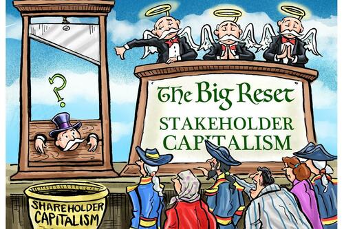
The new fascism is a re-branded philosophy best represented by something called “Stakeholder Capitalism.” It is a term often used by globalists at the World Economic Forum and the head of the WEF, Klaus Schwab. The media friendly definition of Stakeholder Capitalism is:
A form of capitalism in which companies do not only optimize short-term profits for shareholders, but seek long term value creation, by taking into account the needs of all their stakeholders, and society at large.
But who are “all stakeholders” in the opinion of the WEF?
Well, according to Klaus Schwab they are all of human civilization, now and in the future. In other words, the goal of SHC is for corporate leaders and globalist bureaucracy to take responsibility for the entire world, not just their own employees, shareholders and profits. And such leaders would not be acting as individuals, they would be acting as a collective. In other words, SHC requires all major corporations to act as a single unit with a single purpose and a unified collectivist ideology – An ideological monopoly.
As Klaus Schwab states:
“The most important characteristic of the stakeholder model today is that the stakes of our system are now more clearly global. Economies, societies, and the environment are more closely linked to each other now than 50 years ago. The model we present here is therefore fundamentally global in nature, and the two primary stakeholders are as well.
…What was once seen as externalities in national economic policy making and individual corporate decision making will now need to be incorporated or internalized in the operations of every government, company, community, and individual. The planet is thus the center of the global economic system, and its health should be optimized in the decisions made by all other stakeholders.”
The SHC concept is deceptive on its very face because it pretends as if corporations will be held accountable by the public within some form of “business democracy,” as if the public will have a vote on what the corporations do. In reality, it will be corporations telling the public what is acceptable to think and do and corporations in conjunction with governments using their power to punish people who do not agree.
The great magic trick is that these same unified corporations use the shield of “private property” and business rights as a means to control society without repercussions. After all, a primary principle of conservatism and the US constitution is private property rights. So, stepping in to disrupt corporate governance would be violating one of our own beloved ideals. It sounds like a Catch-22, but it’s really not.
As mentioned above, corporations are at their very core a socialist concept: They are created through government charter, handed legal personhood and given special protections from government. They are NOT free market entities, and Adam Smith, the originator of most free market ideals, stood against corporations as destructive and prone to monopoly.
As long as they receive protections from government including monetary stimulus and bailouts, corporations should not enjoy the same private property protections as regular businesses do. They are parasitic creations, alien to the natural business world. In a freedom-based society they would be dismantled to prevent authoritarian outcomes.
Stakeholder Capitalism is also an incredibly arrogant premise because it assumes that corporate leaders have the wisdom or objective intelligence to expand their role beyond business and into social and political spheres. This has already happened in many respects with much chaos created, but open corporate governance is the end game and it is anything but objective or benevolent.
What are some examples of this kind of corporate/political governance (fascism) in action?
How about Big Tech social media censorship leaning HEAVILY against conservatives and liberty activists? How about evidence of collusion between Big Tech companies and government, such as the Biden Administration and the DHS working closely with Twitter and Facebook to actively remove voices and viewpoints they don’t like? How about corporate leaders colluding to destroy conservative based social media competitors like Parler?
How about ESG loans funded by corporate backers such as Blackrock or globalist non-profits like the Rockefeller Foundation?
If all corporate lenders applied ESG to their loan practices, all individuals and businesses would have to adopt leftist social ideologies and dubious environmental claims in order to have access to credit. ESG is a monetary incentive created by corporate elites to keep all other businesses in line. If it continues, ESG could wipe out political opposition to globalism in the span of a single generation.
And, what about the Council For Inclusive Capitalism? This is the most blatant expression of open global fascism I have ever seen, with money elites and politicians working in concert with the UN and even religious leaders like Pope Francis. Their goal is to institute a single centralized world governing platform built around the same agendas outlined in ESG and SHC, making corporations members of a new global council which they refer to as “The Guardians.” They aren’t even trying to hide the conspiracy anymore, it’s right out in the open.
Klaus Schwab takes special care to mention often that global crisis events are the “opportunity” that is needed to push the public into the arms of Stakeholder Capitalism through a nexus point called “The Great Reset.” Meaning, he thinks that widespread fear and desperation must exist (or be engineered) to perpetuate the SHC framework quickly.
Obviously, the globalists are on a shrinking timeline, though it’s hard to say why. They are tearing off the mask faster in the past two years than they have in the previous decade. More than likely they understand to some degree that if they go too slow the public will have time to mount a defense against them.
They will conjure all kinds of distractions and scapegoats to prevent liberty minded people from hitting them back. They’ll aim us at Russia, they’ll aim us at China, they’ll aim us at useful idiots among the leftists. They’ll aim Russia, China and the leftists at us. They will try to send us to war, they will call us insurrectionists, they will call us terrorists, they will say we started the whole collapse and that we are to blame for the world’s ills. None of this matters. What matters is that the globalists at the top pay the price for the harm they cause.
When the head of the snake is removed, only then can we sort out who is to blame; who were the heroes, who were the villains, and who were the idiots. Only then can we rebuild with true freedom in mind.
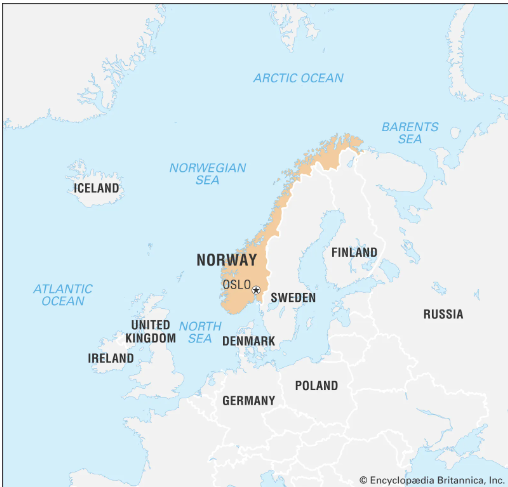
Chief of Defense Eirik Kristoffersen predicts that Norway will be part of the area responsible for mobilizing a joint NATO command center. A final decision will be made during the first half of 2023. NATO currently has a command center in Bussum, Netherlands, which was activated in February as soon as the war began. Kristofferson said that the joint NATO venture is being led by the US Marines – first ones in, last ones out.
Once Sweden and Finland become full NATO members, they will join the joint NATO army. Finland has stated that it wants to be under the control of US forces, which was one of their premises when they decided to join the alliance. The Nordic alliance remains strong, and Norway’s strategic placement will allow it to become the center of operations. With the powerful backing of the world’s most powerful military, NATO’s army will grow. They are preparing.
Posted originally on the conservative tree house on November 10, 2022 | Sundance
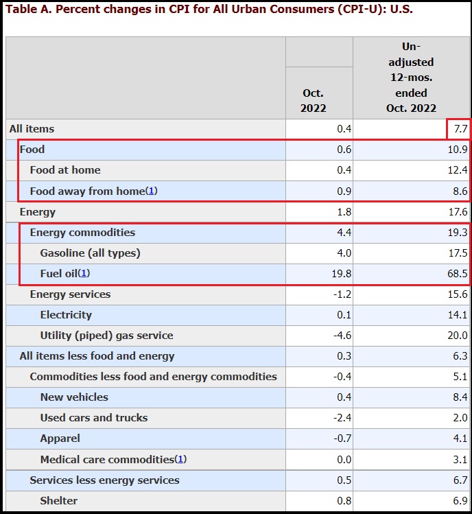
The Bureau of Labor and Statistics (BLS) provides the latest data on consumer prices (inflation) [DATA HERE]. We explained in 2021 how inflation would grow on a month-over-month and year-over-year basis until the calendar became more friendly and the government officials could claim “diminished inflation growth.” Well, we are now entering that phase of economic parseltongue.
October consumer prices increased 0.4% over September. However, we are now comparing year-over-year (Y0Y) inflation to the period where last year’s prices had already skyrocketed, so YoY inflation seems to be moderating at 7.7%, it’s a false premise. {Go Deep}
As expected, the energy-driven consumer inflation in the food sector has arrived. The proverbial field inflation is arriving at the fork, and the October CPI now shows the third wave of food price increases we had previously discussed.
Table 2 Details: Egg prices increased +10.1% last month and now 43% higher than last year. Butter +1.9% last month, 26.7% for year. Margarine +1.3% for month, 47.1% for year. Coffee +1.3% for the month, 15.6% for the year.
Heading into baking season we find flour +0.2% for the month, +24.6% for year. Essentially, as expected, all of the holiday foodstuffs are now rising in price as the increased field and commodity prices hit the store shelves.
Some row crops are starting to moderate in price growth, while dairy products continue rising throughout the fall season. It is going to be painful on the checkbook grocery shopping this holiday season.
On the energy front, home heating oil increased 19.8% in October and is now a whopping 68.5% higher than last October. Unleaded gasoline increased another 3.5% and now is now 20.9% higher than last year (Oct ’21), which was already 40% higher than January 2021.
Food, fuel, electricity, home heating and housing costs continue growing monthly, but give the illusion of moderating when compared to last year.
Food away from home (restaurants etc.) are starting to show the cumulative price impacts for restaurants, hotels and cafeterias. Additionally, as the kids returned to school the lunchroom prices have skyrocketed a jaw-dropping +3.8% for October and +95% compared to last year [Table 2]. Packing lunches for kids is going to become an even more important aspect for the family food budget.
The stock market is happy with the news because the lowered 7.7% (YoY) inflation number, a product of the calendar and nothing else, gives optimism the Fed may moderate the increased federal reserve rate hikes. However, don’t count on it because inflation is easily identified as embedded now. Lemons at the grocery store are now $0.99/each.
Think about that. $1 for a single lemon and roughly 50¢ per egg at the supermarket. A full shopping cart of groceries now easily exceeding $200. This is devastating for those on fixed incomes and blue-collar workers.
Wages are nowhere near keeping up with this level of price increase.
(CNBC) The consumer price index rose less than expected in October, an indication that while inflation is still a threat to the U.S. economy, pressures could be starting to cool.
The index, a broad-based measure of goods and services costs, increased 0.4% for the month and 7.7% from a year ago, according to a Bureau of Labor Statistics release Thursday. Respective estimates from Dow Jones were for rises of 0.6% and 7.9%.
Excluding volatile food and energy costs, so-called core CPI increased 0.3% for the month and 6.3% on an annual basis, compared with respective estimates of 0.5% and 6.5%.
A 2.4% decline in used vehicle prices helped bring down the inflation figures. Apparel prices fell 0.7% and medical care services were lower by 0.6%.
“The report overstates the case that inflation is coming in, but it makes a case inflation is coming in,” said Mark Zandi, chief economist at Moody’s Analytics. “It’s pretty clear that inflation has definitely peaked and is rolling over. All the trend lines suggest that it will continue to moderate going forward, assuming that nothing goes off the rails.” (read more)
The Biden energy policy is the root of the consumer inflation. Nothing will happen to moderate overall consumer inflation on Main Street until energy policy changes.
Additionally, with the 2022 election in the rear-view mirror, we should start to see layoffs and unemployment increasing now. The bureaucrats will now let the recession become evident.
COMMENT from Thailand: In Thailand, for the whole 2020, there is only 61 Covid deaths. Few months after mass vaccination there is 20000 “Covid” deaths. This year, I believed that there is an explosion of COVID illnesses and deaths, just like Canada. And the authority is keeping a tight lip about it. Look like 2022 desease cycle is driven by the COVID Varients.
DC
REPLY: All of the death I personally know of are ONLY from those who were vaccinated. The NY Supreme Court ordered back pay to those who were fired for refusing the vaccines stating that the vaccine neither prevented anyone from getting COVID nor spreading it. It was a total PR routine and the politicians merely got their pockets filled thanks to bribes.
COMMENT From Brazil: So, about the Brazilian Elections. The Brazilian military (DoD) were not allowed to access the source code by the Supreme Court. The conclusion, the fraud is guaranteed, as the lack of transparency. I wouldn’t want to be in Lula’s shoes. Now, everybody knows. There was a huge fraud against Bolsonaro, because nobody voted in Lula. Unbelievable, the world will not recover from this, the thing is going into free fall. When the military cannot do its job, something is very rotten, they have no authority within their own country, so where does this external power or interference come from? King regards, R.
REPLY: Bolsonaro had to be removed from office the same as Trump, Putin, and Jinping. I have a video clip someone took at the Davos WEF meeting in 2019 where Bolsonaro said these people are insane. The EU organized a rigged election in Italy to get rid of Silvio Berlusconi. The EU rigged the Scottish separatist vote as well. The EU rules that Catalonia has no right to separate.
We do not live in a world where the right to vote is truly respected. Bolsonaro had to go for the WEF was out to remove him because he stood against their climate change agenda. There is nothing we can do about this. It will play out and blow up in everyone’s face.
It is rare for a celebrity to speak out against the agenda. Pink Floyd’s Roger Waters has reached a level of fame where he can question the status quo as his legacy is sealed. Waters called Biden a “war criminal” for encouraging the war in Ukraine. “This war is about the action and reaction of NATO pushing right up to the Russian border, which they promised they wouldn’t do when Gorbachev negotiated the withdrawal of the USSR,” Waters declared. Amazing how a musician understands the situation better than politicians.
CNN attempted to argue with Waters, but he held firm. The reporter attempted and failed to belittle Waters by saying he should see Russia as the enemy as his father died in the last world war. However, that is precisely what Waters and any sensible human are aiming to avoid – another world war. “Don’t forget 23 million Russians died protecting you and me from the Nazis,” Waters said.
He then asked the reporter what he thought America would do if China began to line up on the US border. We all know the answer to that question. Imagine if China placed nuclear weapons in or near Canada and Mexico? The nuclear apocalypse would have already happened.
Many hold the same views as Roger Waters, but they are too afraid to speak up. The average person, who may not tune into political commentary, will listen to celebrities when they speak. The problem becomes the fear of cancelation. It is career suicide to question the current agenda. Pink Floyd cannot be canceled; they’ve been popular for far too many decades. The left “hippies” of the past are nothing like the hipsters today who encourage war and echo the voices of the elite.
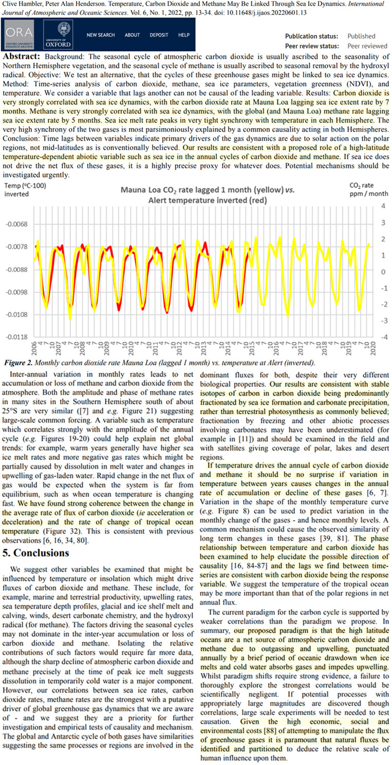
Annual carbon dioxide (CO2) and methane (CH4) change rates lag behind changes in sea ice extent by 7 months and 5 months, respectively. This robust correlation is consistent with the conclusion that CO2 (and CH4) changes are responsive to temperature, not the other way around.
It is commonly believed that the annual “squiggle” of the Mauna Loa CO2 cycle variations are driven by hemispheric seasonal contrasts in terrestrial photosynthesis.
But scientists (Hambler and Henderson, 2022) instead find it is variation high latitude temperatures affecting sea ice extent changes that dominate as drivers of the CO2 (and methane) annual fluxes, not photosynthesis.
They affirm temperature (T) changes lead CO2 change rates by about 7-10 months, suggesting the causality direction is T→CO2, and not CO2→T.
Temperature also drives sea ice peak melt vs. accumulation rates. This cause-effect directionality can also be clearly seen in analyses of sea ice flux vs. annual CO2 rate changes.
“The phase relationship between temperature and carbon dioxide has been examined to help elucidate the possible direction of causality and the lags we find between timeseries are consistent with carbon dioxide being the response variable.”
“Carbon dioxide is very strongly correlated with sea ice dynamics, with the carbon dioxide rate at Mauna Loa lagging sea ice extent rate by 7 months. Methane is very strongly correlated with sea ice dynamics, with the global (and Mauna Loa) methane rate lagging sea ice extent rate by 5 months. Sea ice melt rate peaks in very tight synchrony with temperature in each Hemisphere.”
I have created this site to help people have fun in the kitchen. I write about enjoying life both in and out of my kitchen. Life is short! Make the most of it and enjoy!
This is a library of News Events not reported by the Main Stream Media documenting & connecting the dots on How the Obama Marxist Liberal agenda is destroying America

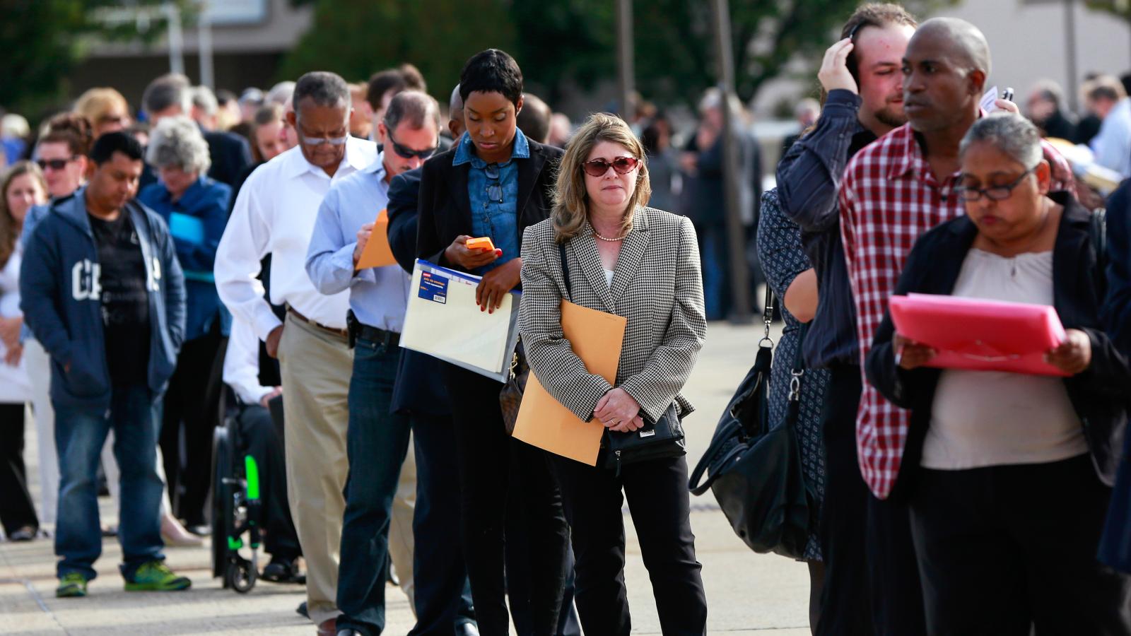


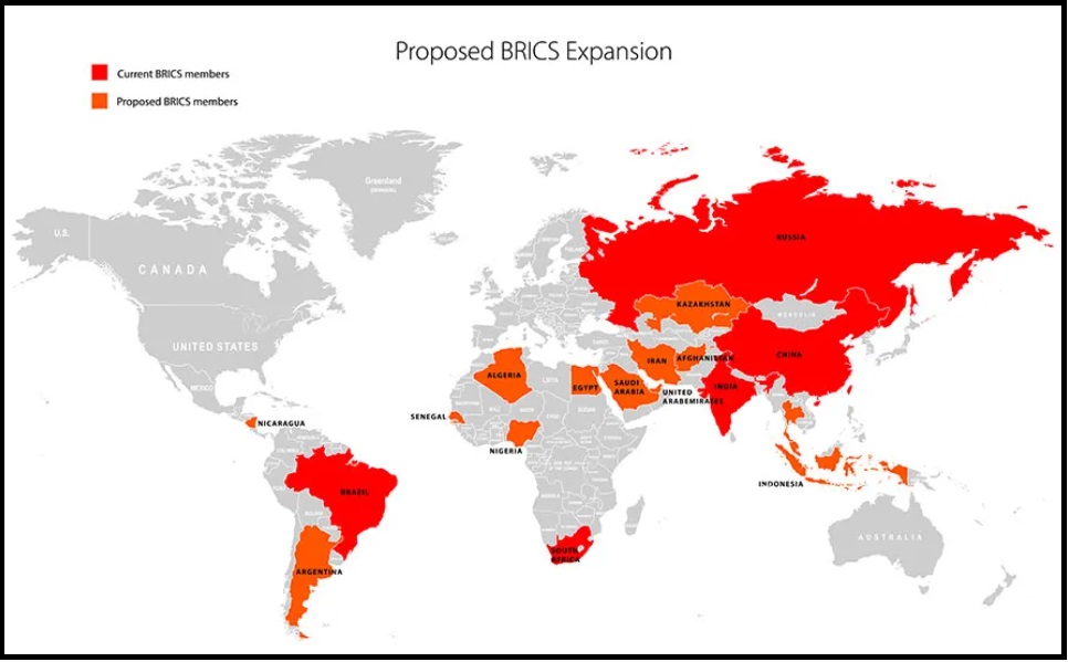
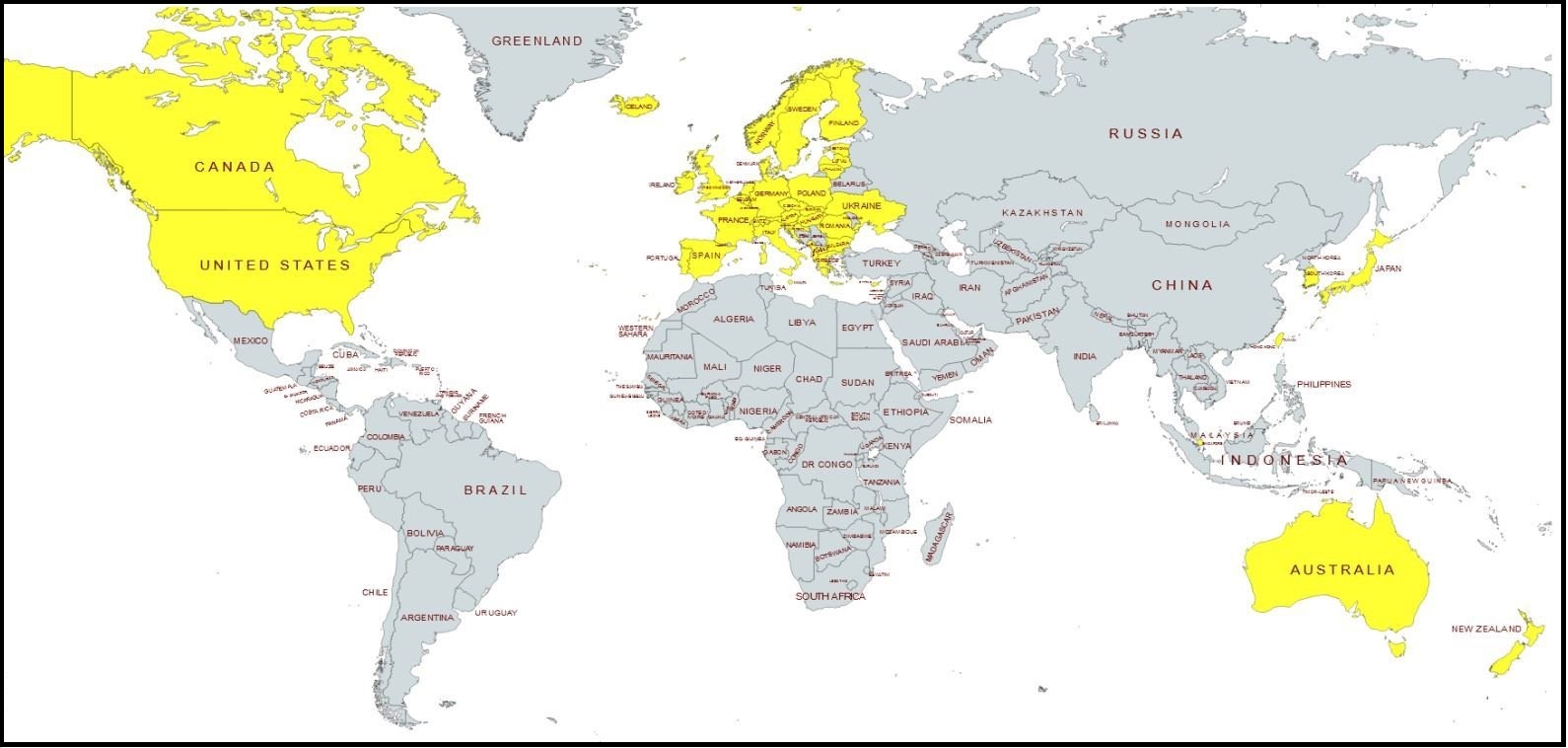
 Figure 1: Incremental warming effect of CO2 alone [1]
 Figure 2: Typical grid used in climate models [2]
 Figure 3: Global weather stations circa 1885 [3]
 Figure 4: How grid cells interact with adjacent cells [4]
 Figure 5: IPCC models in forecast mode for the Mid-Troposphere vs Balloon and Satellite observations [5]
 Figure 6: Comparison of the IPCC model predictions with those from a harmonic analytical model [6]


